Chapter 3 Linear Model Selection & Regularisation

In the previous chapter we discussed cross-validation (CV) as a procedure for estimating the out-of-sample performance of models of the same form, but different complexity, where each model was considered a separate hypothesised representation of the underlying function \(f\) mapping all the explanatory variables (features) to the dependent (target) variable. In the following sections we will start by fitting a linear model, with the focus then on variable selection, i.e. deciding which features to include in the model. Instead of deciding on the model “settings” beforehand – which we will in later chapters come to know as hyperparameters – we will rather adjust the fitted model parameters by means of regularisation, also referred to as shrinkage methods. Following that, we will cover dimension reduction methods.

This chapter is loosely based on chapter 6 of James et al. (2013) and chapter 3 of Hastie et al. (2009) and assumes some basic knowledge of linear regression models.

3.1 Linear regression models

Although few real-world relationships can be considered truly linear, the linear model offers some distinct advantages, most notably in the clear interpretation of features³. Furthermore, they often perform surprisingly well on a range of problems.

For some real-valued output \(Y\) and input vector \(\boldsymbol{X}' = [X_1, X_2, \ldots, X_p]\), the model is defined as:

\[\begin{equation} Y = \beta_0 + \sum_{j=1}^p\beta_jX_j + \epsilon, \tag{3.1} \end{equation}\]

where \(\epsilon \sim N(0, \sigma^2)\).

The most popular method of estimating the regression parameters based on the training set \(\mathcal{D}=\{\boldsymbol{x}_i, y_i\}_{i=1}^n\), is ordinary least squares (OLS), where we find the coefficients \(\boldsymbol{\beta} = [\beta_0, \beta_1, \ldots, \beta_p]'\) to minimise the residual sum of squares

\[\begin{equation} RSS(\boldsymbol{\beta}) = \sum_{i=1}^n\left( y_i - \beta_0 - \sum_{j=1}^px_{ij}\beta_j \right)^2, \tag{3.2} \end{equation}\]

noting that this does not imply any assumptions on the validity of the model.

To minimise \(RSS(\boldsymbol{\beta})\), let us first write (3.1) in matrix form:

\[\begin{equation} _n\boldsymbol{Y}_1 = {}_n\boldsymbol{X}_{(p+1)} \boldsymbol{\beta}_1 + {}_n\boldsymbol{\epsilon}_1, \tag{3.3} \end{equation}\]

where the first column of \(\boldsymbol{X}\) is \(\boldsymbol{1}:n\times1\).

Now we can write

\[\begin{equation} RSS(\boldsymbol{\beta}) = \left(\boldsymbol{y} - \boldsymbol{X}\boldsymbol{\beta} \right)'\left(\boldsymbol{y} - \boldsymbol{X}\boldsymbol{\beta} \right), \tag{3.4} \end{equation}\]

which is a quadratic function in the \(p+1\) parameters. Differentiating with respect to \(\boldsymbol{\beta}\) yields

\[\begin{align} \frac{\partial RSS}{\partial \boldsymbol{\beta}} &= -2\boldsymbol{X}'\left(\boldsymbol{y} - \boldsymbol{X}\boldsymbol{\beta} \right) \\ \frac{\partial^2 RSS}{\partial \boldsymbol{\beta}\partial \boldsymbol{\beta}'} &= 2\boldsymbol{X}'\boldsymbol{X} \tag{3.5} \end{align}\]

If \(\boldsymbol{X}\) is of full column rank – a reasonable assumption when \(n \geq p\) – then \(\boldsymbol{X}'\boldsymbol{X}\) is positive definite. We can then set the first derivative to zero to obtain the unique solution

\[\begin{equation} \hat{\boldsymbol{\beta}} = \left(\boldsymbol{X}'\boldsymbol{X}\right)^{-1}\boldsymbol{X}'\boldsymbol{y} \tag{3.6} \end{equation}\]

These coefficient estimates define a fitted linear regression model. The focus of this section is on methods for improving predictive accuracy, therefore we will not cover inference on the regression parameters or likelihood ratio tests here.

The following section instead answers the question: “How can one simplify a regression model, either by removing covariates or limiting their contribution, in order to improve predictive performance?” Before delving into regularisation methods, we will briefly note the existence of subset selection methods.

Subset selection

Although subject to much criticism, there are some specific conditions in which subset selection could yield satisfactory results, for instance when \(p\) is small and there is little to no multicollinearity. This selection can generally be done in two ways:

1. Best subset selection

This approach identifies the best fitting model across all \(2^p\) combinations of predictors, by first identifying the best \(k\)-variable model \(\mathcal{M}_k\) according to RSS, for all \(k = 1, 2, \ldots, p\).

2. Stepwise selection

Starting with either the null (forward stepwise) or saturated (backward stepwise) model, predictors are sequentially added or removed respectively according to some improvement metric. One can also apply a hybrid method, which considers both adding and removing a variable at each step.

Typically, either Mallow’s \(C_p\), AIC, BIC, or adjusted \(R^2\) is used for model comparison in subset selection.

Because subset selection is a discrete process, with variables either retained or discarded, it often exhibits high variance, thereby failing to reduce the test MSE. Regularisation offers a more continuous, general-purpose and usually quicker method of controlling model complexity.

Note that although the linear model is used here to illustrate the theory of regularisation, it can be applied to any parametric model.

3.2 \(L_1\) and \(L_2\) regularisation

As an alternative to using least squares, we can fit a model containing all \(p\) predictors using a technique that constrains or regularises the coefficient estimates, or equivalently, that shrinks the coefficient estimates towards zero by imposing a penalty on their size. Hence, regularisation is also referred to as shrinkage methods. This approach has the effect of significantly reducing the coefficient estimates’ variance, thereby reducing the variance component of the total error. The two best-known techniques for shrinking the regression coefficients towards zero, are ridge regression and the lasso.

3.2.1 Ridge regression – \(L_2\)

Ridge regression was initially developed as a method of dealing with highly correlated predictors in regression analysis. Instead of finding regression coefficients to minimise (3.2), the ridge coefficients minimise a penalised residual sum of squares:

\[\begin{equation} \hat{\boldsymbol{\beta}}_R = \underset{\boldsymbol{\beta}}{\text{argmin}}\left\{ \sum_{i=1}^n\left( y_i - \beta_0 - \sum_{j=1}^px_{ij}\beta_j \right)^2 + \lambda \sum_{j=1}^p\beta_j^2 \right\}. \tag{3.7} \end{equation}\]

The complexity parameter \(\lambda \geq 0\) controls the amount of shrinkage. As \(\lambda\) increases, the coefficients are shrunk towards zero, whilst \(\lambda = 0\) yield the OLS. Neural networks also implement regularisation by means of penalising the sum of the squared parameters; in this context it is referred to as weight decay.

The term “\(L_2\) regularisation”, also stylised as \(\ell_2\), arises because the regularisation penalty is based on the \(L_2\) norm⁴ of the regression coefficients. The \(L_2\) norm of a vector \(\boldsymbol{\beta}\) is given by \(||\boldsymbol{\beta}||_2 = \sqrt{\sum_{i=1}^p \beta_i^2}\).

The optimisation problem in (3.7) can also be written as

\[\begin{equation} \hat{\boldsymbol{\beta}}_R = \underset{\boldsymbol{\beta}}{\text{argmin}} \sum_{i=1}^n\left( y_i - \beta_0 - \sum_{j=1}^px_{ij}\beta_j \right)^2, \\ \text{subject to } \sum_{j=1}^p\beta_j^2 \leq \tau, \tag{3.8} \end{equation}\]

where \(\tau\), representing the explicit size constraint on the parameters, has a one-to-one correspondence with \(\lambda\) in (3.7).

When collinearity exists in a linear regression model the regression coefficients can exhibit high variance, such that correlated predictors, which carry similar information, can have large coefficients with opposite signs. Imposing a size constraint on the coefficients addresses this problem.

It is important to note that since ridge solutions are not equivariant under scaling of the inputs⁵, the inputs are generally standardised before applying this method. Note also the omission of \(\beta_0\) in the penalty term. Whereas the regression coefficients depend on the predictors in the model, the bias term is a constant independent of the predictors, i.e. it is a property of the data that does not change as variables are added or removed. Now, if the inputs are standardised such that each \(x_{ij}\) is replaced by \(\frac{x_{ij} - \bar{x}_j}{s_{x_j}}\), then \(\beta_0\) is estimated by \(\bar{y} = \frac{1}{n}\sum_{i=1}^n y_i\) and \(\beta_1, \ldots, \beta_p\) are estimated by a ridge regression without an intercept, using the centered \(x_{ij}\). The same applies to the lasso discussed in the following section.

Assuming this centering has been done, the input matrix \(\boldsymbol{X}\) then becomes \(n\times p\), such that the penalised RSS, now viewed as a function of \(\lambda\), can be written as

\[\begin{equation} RSS(\lambda) = \left(\boldsymbol{y} - \boldsymbol{X}\boldsymbol{\beta} \right)'\left(\boldsymbol{y} - \boldsymbol{X}\boldsymbol{\beta} \right) + \lambda\boldsymbol{\beta}'\boldsymbol{\beta}, \tag{3.9} \end{equation}\]

yielding the ridge regression solution

\[\begin{equation} \hat{\boldsymbol{\beta}} = \left(\boldsymbol{X}'\boldsymbol{X} + \lambda\boldsymbol{I}\right)^{-1}\boldsymbol{X}'\boldsymbol{y} \tag{3.10}, \end{equation}\]

where \(\boldsymbol{I}\) is the \(p \times p\) identity matrix.

Equation (3.10) shows that the ridge regression addresses singularity issues that can arise when the predictor variables are highly correlated. The regularisation term ensures that even if \(\boldsymbol{X}'\boldsymbol{X}\) is singular, the modified matrix \(\boldsymbol{X}'\boldsymbol{X} + \lambda\boldsymbol{I}\) is guaranteed to be non-singular, allowing for stable and well-defined solutions to be obtained.

Although all of the above can be neatly explored via simulated examples, our focus will now move away from this controlled environment and towards using R packages to implement this methodology on some real-world data.

3.2.2 Example 2 – Prostate cancer

This dataset formed part of the now retired ElemStatLearn R package; it’s details can be found here. The goal is to model the (log) prostate-specific antigen (lpsa) for men who were about to receive a radical prostatectomy, based on eigth clinical measurements. The data only contain 97 observations, 30 of which are set aside for testing purposes.

Looking at the correlations displayed in Figure 3.1, we see that all the features are positively correlated with the response variable, ranging from relatively weak (0.23) to relatively strong (0.73) correlation. We also observe some strong correlation between features, which could be of concern for a regression model. Note! svi and gleason are actually binary and ordinal variables respectively, but we will treat them as numeric for the sake of simplicity in this illustration.

library(corrplot) #For correlation plot

dat_pros <- read.csv('data/prostate.csv')

# Extract train and test examples and drop the indicator column
train_pros <- dat_pros[dat_pros$train, -10]
test_pros <- dat_pros[!dat_pros$train, -10]

corrplot(cor(train_pros), method = 'number', type = 'upper')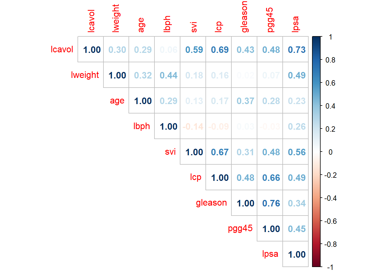

Figure 3.1: Correlation plot for the prostate cancer data.

Next, we standardise the predictors and fit a saturated linear model.

library(kableExtra) 
library(broom) #For nice tables

# Could do the following neatly with tidyverse, this is a MWE
y <- train_pros[, 9]  #9th column is target variable
x <- train_pros[, -9] 
x_stand <- scale(x) #standardise for comparison
train_pros_stand <- data.frame(x_stand, lpsa = y)

# Fit lm using all features
lm_full <- lm(lpsa ~ ., train_pros_stand)
lm_full %>% 
  tidy() %>%
  kable(digits = 2, caption = 'Saturated linear model fitted to the prostate cancer dataset (features standardised).')

Table 3.1: Saturated linear model fitted to the prostate cancer dataset (features standardised).

term	estimate	std.error	statistic	p.value
(Intercept)	2.45	0.09	28.18	0.00
lcavol	0.72	0.13	5.37	0.00
lweight	0.29	0.11	2.75	0.01
age	-0.14	0.10	-1.40	0.17
lbph	0.21	0.10	2.06	0.04
svi	0.31	0.13	2.47	0.02
lcp	-0.29	0.15	-1.87	0.07
gleason	-0.02	0.14	-0.15	0.88
pgg45	0.28	0.16	1.74	0.09

The features gleason, age, and possibly pgg45 and lcp are non-significant in this model, although note that these variables in particular were highly correlated with each other. This example also illustrates the adverse effect that this multicollinearity can have on a regression model. Even though lcp was observed to have a fairly strong positive linear relationship with the response variable (r = 0.49, third highest of all features), the coefficient estimate is in fact negative, relatively significantly (p = 0.07)! Likewise, even though age is positively correlated with lpsa (r = 0.23), its coefficient estimate is negative.

Let us now apply \(L_2\) regularisation using the glmnet package in R. See section 3.3 for the discussion of the \(\alpha\) parameter. For now, note that \(\alpha = 0\) corresponds to ridge regression.

library(glmnet)
ridge <- glmnet(x, y, alpha = 0, standardize = T,
                lambda = exp(seq(-4, 5, length.out = 100)))
plot(ridge, xvar = 'lambda', label = T)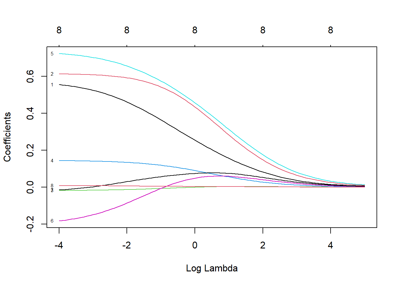

Figure 3.2: Coefficient profiles for ridge regression on the prostate cancer dataset

Here we see how the coefficients vary as \(\log(\lambda)\) is increased, whilst the labels at the top indicate the number of nonzero coefficients for various values of \(\log(\lambda)\). Note that none of the coefficients actually equal zero, illustrating that ridge regression does not necessarily perform variable selection per se.

In Figure 3.2 we observe that the initially negative coefficient for lcp \((\beta_6)\) becomes both positive and more significant, relative to the other predictors. Therefore, the notion of “coefficients shrinking towards zero” is a slight misnomer, or perhaps an oversimplification of the effect \(L_2\) regularisation has. Eventually, as \(\lambda \to \infty\) (or, equivalently, \(\tau \to 0\) as shown in (3.8)), all coefficients will indeed be forced towards zero. However, the ideal model will usually correspond to a level of \(\lambda\) that allows stronger predictors to be more prominent by diminishing the effect of their correlates.

So, how do we determine the appropriate level of \(\lambda\)? By viewing this tuning parameter as a proxy for complexity and applying the same approach as in Chapter 2, we can use CV with the MSE as loss function to identify optimal complexity.

#Apply 10-fold CV
set.seed(1)
ridge_cv <- cv.glmnet(as.matrix(x), y, #this function requires x to be a matrix
                      alpha = 0, nfolds = 10, type.measure = 'mse', standardize = T,
                      lambda = exp(seq(-4, 5, length.out = 100))) #Default lambda range doesn't cover minimum
plot(ridge_cv)
abline(h = ridge_cv$cvup[which.min(ridge_cv$cvm)], lty = 2)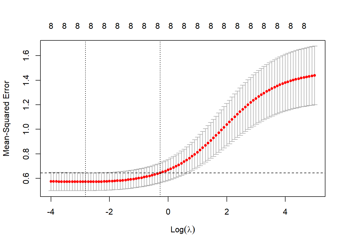

Figure 3.3: 10-fold CV MSEs as a function of \(\log(\lambda)\) for ridge regression applied to the prostate cancer dataset

Figure 3.3 shows the CV errors (red dots), with the error bars indicating the extent of dispersion of the MSE across folds, the default display being one standard deviation above and below the average MSE. Two values of the tuning parameter are highlighted: the one yielding the minimum CV error (lambda.min), and the one corresponding to the most regularised model such that the error is within one standard error of the minimum (lambda.1se), which has been indicated on this plot with the horizontal dashed line.

The choice of \(\lambda\) depends on various factors, including the size of the data set, the length of the resultant error bars, and the profile of the coefficient estimates. In Figure 3.2 we saw that a more “reasonable” representation of the coefficients is achieved when \(\log(\lambda)\) is closer to zero, rather than at the minimum CV MSE. Showing this explicitly, below we see that the coefficients corresponding to lambda.min (left) still preserves the contradictory coefficient sign for lcp, whereas lambda.1se (right) rectifies this whilst mostly maintaining the overall relative importance across the features, hence we will use the latter.

round(cbind(coef(ridge_cv, s = 'lambda.min'), coef(ridge_cv, s = 'lambda.1se')), 3)

## 9 x 2 sparse Matrix of class "dgCMatrix"
##                 s1     s1
## (Intercept)  0.173 -0.181
## lcavol       0.515  0.284
## lweight      0.606  0.470
## age         -0.016 -0.002
## lbph         0.140  0.099
## svi          0.696  0.492
## lcp         -0.140  0.038
## gleason      0.007  0.071
## pgg45        0.008  0.004

Note that although some predictors have almost been removed, these coefficients are still nonzero. Therefore, the ridge regression will include all \(p\) predictors in the final model. The CV MSE for the chosen model, which is an estimate of out-of-sample performance, is 0.645.

Before using the ridge regression to predict values for the test set, we will first consider the lasso as an approach for variable selection.

3.2.3 The Lasso – \(L_1\)

Lasso is an acronym that stands for least absolute shrinkage and selection operator. It is another form of regularisation that, similar to ridge regression, attempts to minimise a penalised RSS. However, the constraint is slightly different:

\[\begin{equation} \hat{\boldsymbol{\beta}}_L = \underset{\boldsymbol{\beta}}{\text{argmin}} \sum_{i=1}^n\left( y_i - \beta_0 - \sum_{j=1}^px_{ij}\beta_j \right)^2, \\ \text{subject to } \sum_{j=1}^p|\beta_j| \leq \tau. \tag{3.11} \end{equation}\]

Or, written in its Lagrangian form:

\[\begin{equation} \hat{\boldsymbol{\beta}}_L = \underset{\boldsymbol{\beta}}{\text{argmin}}\left\{ \sum_{i=1}^n\left( y_i - \beta_0 - \sum_{j=1}^px_{ij}\beta_j \right)^2 + \lambda \sum_{j=1}^p |\beta_j| \right\}. \tag{3.12} \end{equation}\]

Again we can see that the equivalent name “\(L_1\) regularisation” arises from the fact that the penalty is based on the \(L_1\) norm⁶ \(||\boldsymbol{\beta}||_1 = \sum_{i=1}^p |\beta_i|\).

This constraint on the regression parameters makes the solutions nonlinear in the \(y_i\), such that there is no closed form expression for \(\hat{\boldsymbol{\beta}}_L\) like there is for the ridge estimate, except in the case of orthonormal covariates. Computing the lasso estimate is a quadratic programming problem, although efficient algorithms have been developed to compute the solutions as a function of \(\lambda\) at the same computational cost as for ridge regression. These solutions are beyond the scope of this course.

Note that if we let \(\tau > \sum_{j=1}^p|\hat{\beta}^{LS}_j|\), where \(\hat{\beta}^{LS}_j\) denotes the least squares estimates, then the lasso estimates are exactly equal to the least squares estimates. If, for example, \(\tau = \frac{1}{2} \sum_{j=1}^p|\hat{\beta}^{LS}_j|\), then the least squares coefficients are shrunk by 50% on average. However, the nature of the shrinkage is not obvious.

When comparing ridge regression with the lasso, we see that the nature of the constraints yield different trajectories for \(\hat{\boldsymbol{\beta}}\) as \(\lambda\) increases/\(\tau\) decreases:

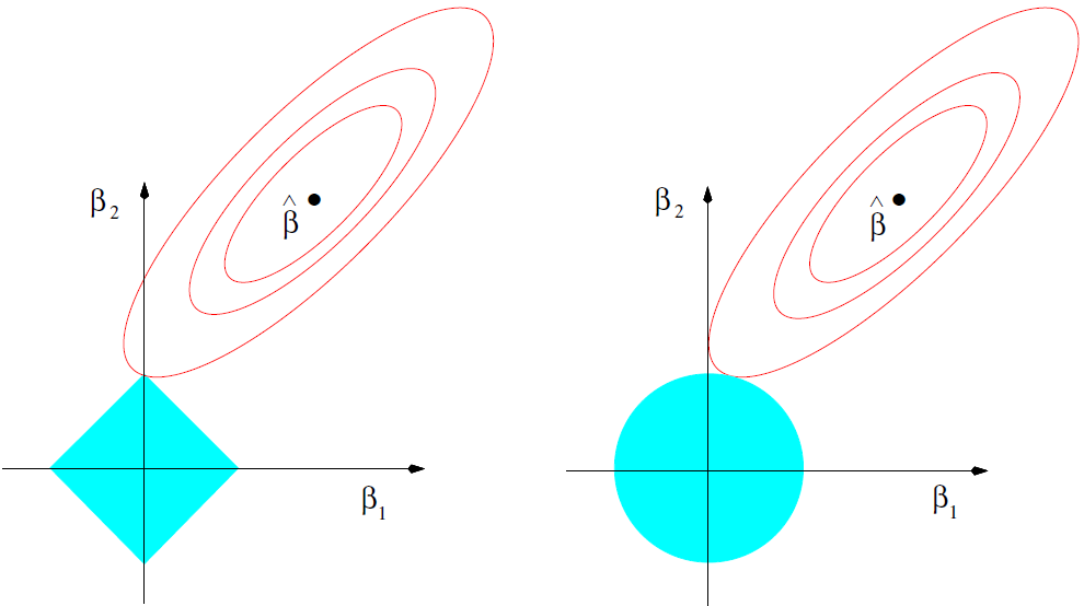
Figure 3.4: Estimation picture for the lasso (left) and ridge regression (right). Shown are contours of the error and constraint functions. The solid blue areas are the constraint regions \(|\beta_1| + |\beta_2| \leq \tau\) and \(\beta_1^2 + \beta_2^2 \leq \tau^2\), respectively, while the red ellipses are the contours of the least squares error function. Source: Hastie et al. (2009), p. 71.

As the penalty increases, the lasso constraint sequentially forces the coefficients across the p dimensions onto their respective axes. Let us return to the previous example to illustrate this effect.

3.2.4 Example 2 – Prostate cancer (continued)

Applying \(L_1\) regularisation via glmnet follows exactly the same process as for ridge regression, except that we now set \(\alpha = 1\) within the glmnet() function.

library(glmnet)
lasso <- glmnet(x, y, alpha = 1, standardize = T)
plot(lasso, xvar = 'lambda', label = T)

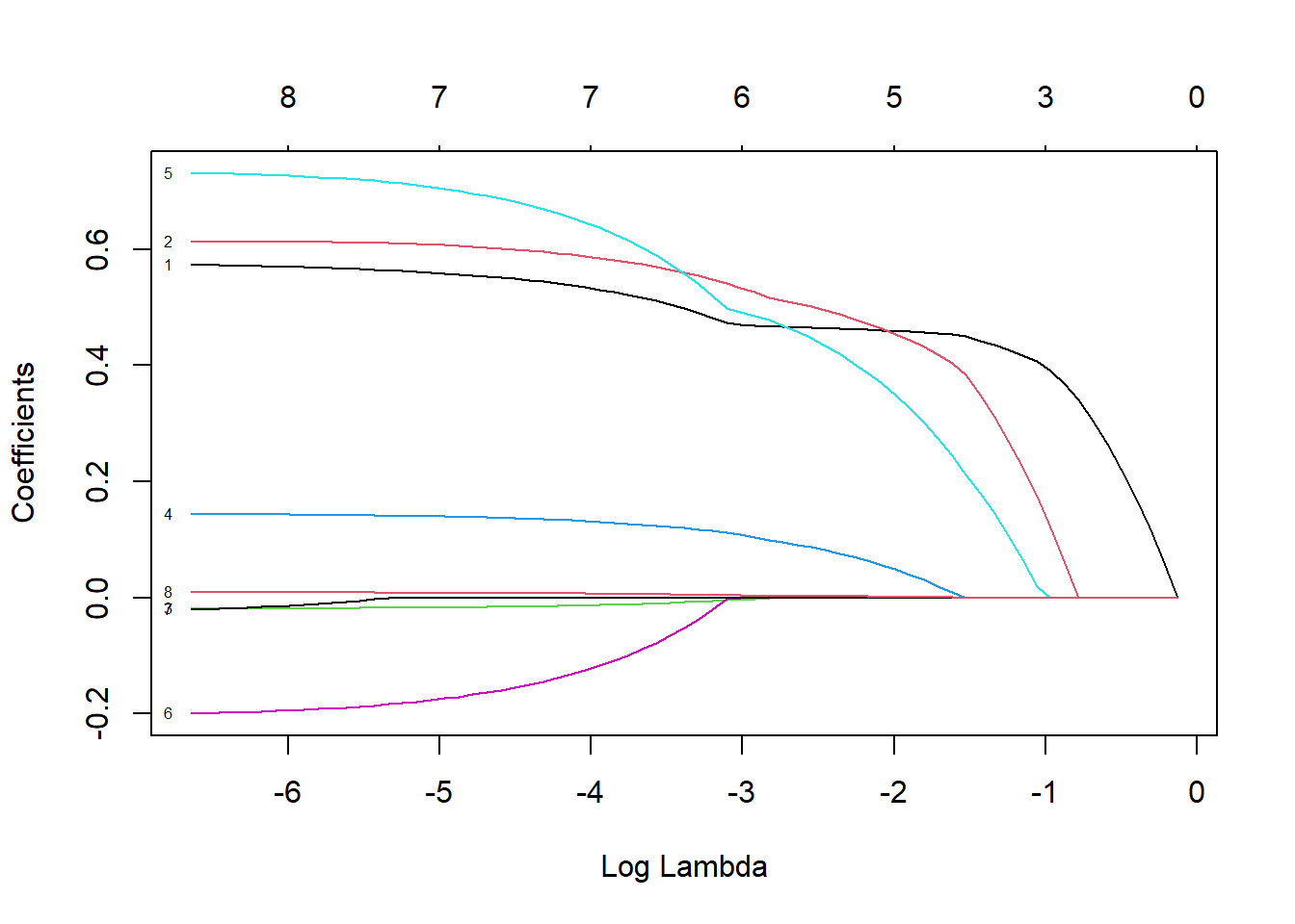
Figure 3.5: Coefficient profiles for lasso regression on the prostate cancer dataset

Figure 3.5 shows the coefficients shrinking and equaling zero as the regularisation penalty increases, as opposed to gradually decaying as in ridge regression, thereby performing variable selection in the process. Interestingly, here it seems that one of the first variables excluded from the model is lcp, although it is quite difficult to see, even for this small example where \(p=8\). In order to determine which variables should be (de)selected, we will again implement CV using the MSE as loss function.

#Apply 10-fold CV
set.seed(1)
lasso_cv <- cv.glmnet(as.matrix(x), y, #this function requires x to be a matrix
                      alpha = 1, nfolds = 10, type.measure = 'mse', standardize = T)
plot(lasso_cv)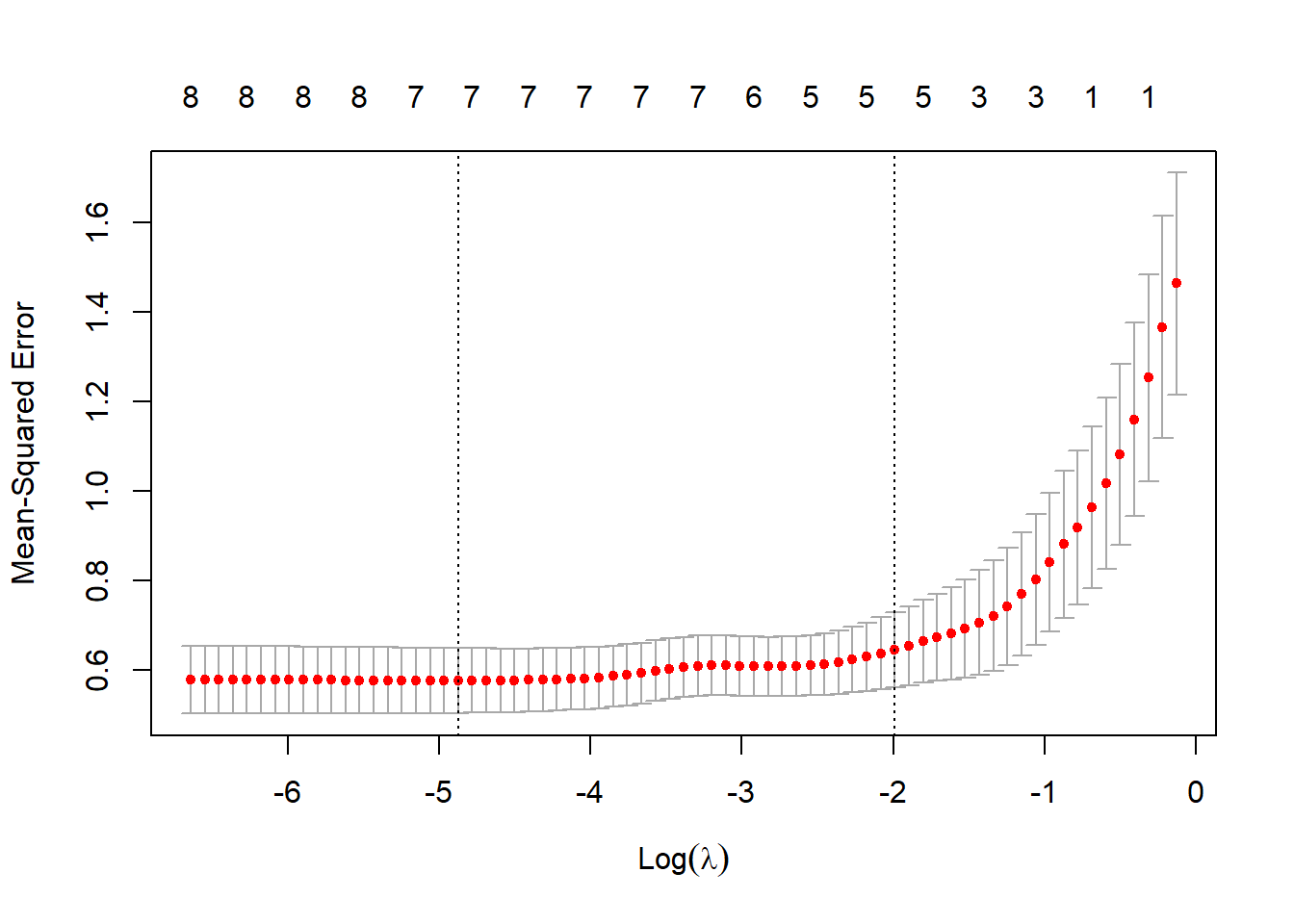

Figure 3.6: 10-fold CV MSEs as a function of \(\log(\lambda)\) for lasso regression applied to the prostate cancer dataset

We can now achieve a notably simpler model where three of the eight coefficients have been shrunk to zero by once again selecting the penalty corresponding to the largest MSE within one standard error of the minimum MSE, as opposed to the minimum MSE where the contradictory estimates will clearly still remain.

round(coef(lasso_cv, s = 'lambda.1se'), 3)

## 9 x 1 sparse Matrix of class "dgCMatrix"
##                s1
## (Intercept) 0.083
## lcavol      0.459
## lweight     0.454
## age         .    
## lbph        0.048
## svi         0.349
## lcp         .    
## gleason     .    
## pgg45       0.001

Once again, the CV MSE for the chosen model is 0.645.

At this point we have defined a new \(\hat{f}\), which is ultimately still a linear model with slightly adjusted coefficient estimates. We can now compare these different versions of the proposed linear model – i.e. the OLS, ridge and lasso models – by looking at their CV MSE’s and selecting the one that performed best. In this instance there is very little difference between the two regularised models, therefore we would favour the more parsimonious model (lasso). As a way of “grading” our decision, we will now take a peek at each model’s performance on the test set, shown in Table 4.3.

To be clear: the test set should NOT be used to inform the choice of model parameters. This decision should be made before using the test set, which is then used to measure the selected model’s fit. Below we are calculating the test MSE for each model for illustrative purposes, in essence evaluating three different hypothetical decisions that had already been made.

test_y <- test_pros[, 9]
test_x <- as.matrix(test_pros[, -9]) #need to extract just the x's for glmnet predict function

test_x_stand <- scale(test_x) #standardise for lm
test_pros_stand <- data.frame(test_x_stand, lpsa = test_y)

#Yhats
ols_pred <-predict(lm_full, test_pros_stand)
ridge_pred <- predict(ridge_cv, test_x, s = 'lambda.1se') 
lasso_pred <- predict(lasso_cv, test_x, s = 'lambda.1se') 

#Test MSEs
ols_mse <- mean((test_y - ols_pred)^2)
ridge_mse <- mean((test_y - ridge_pred)^2)
lasso_mse <- mean((test_y - lasso_pred)^2)

comparison_table <- data.frame(
  Model = c('OLS', 'Ridge', 'Lasso'),
  MSE = c(ols_mse, ridge_mse, lasso_mse)
)

kable(comparison_table, digits = 3,
      caption = 'Prostate cancer data test set MSEs for the saturated, L2-regularised, and L1-regularised linear models.')

(#tab:lm_comp)Prostate cancer data test set MSEs for the saturated, L2-regularised, and L1-regularised linear models.

Model	MSE
OLS	0.549
Ridge	0.509
Lasso	0.454

The final results show that the unregularised linear model performed worst, and the lasso performed best in this example. It should be noted that the accuracy of these predictions in context of the application should always be evaluated in consultation with the subject experts, i.e. the oncologist in this instance.

3.3 Elastic-net

Although both of the regularisation approaches above can be effective in certain situations, each has its limitations: Lasso struggles when predictors are highly correlated, often selecting only one variable from a group while ignoring others. Ridge, on the other hand, retains all predictors but does not perform automatic variable selection. The elastic-net penalty attempts to address these issues by incorporating both \(L_1\) and \(L_2\) penalties, providing a balance between sparsity and stability. First proposed by Zou & Hastie (2005), the elastic-net penalty term is defined as follows:

\[\begin{equation} \text{penalty} = \lambda \left[ (1-\alpha)\left(\sum_{j=1}^p \beta_j^2\right) + \alpha\left(\sum_{j=1}^p |\beta_j|\right) \right] \tag{3.13} \end{equation}\]

Note that the \(\alpha\) terms have actually been swapped around here in order to correspond with the application in glmnet. The elastic-net selects variables like the lasso, and shrinks together the coefficients of correlated predictors like ridge. The effect of \(\alpha\) on the constraint function is illustrated in Figure 3.7.

#Set up a range of alphas between 0 and 1
alphas <- seq(0, 1, 0.1)

for(alpha in alphas){
  beta1 <- beta2 <- seq(-1, 1, 0.01) 
  grid <- expand.grid(beta1 = beta1, beta2 = beta2)
  
  #Define elastic-net constraint
  tau <- (1 - alpha) * (grid$beta1^2 + grid$beta2^2) + alpha * (abs(grid$beta1) + abs(grid$beta2))
  tau_matrix <- matrix(tau, nrow = length(beta1))
  
  #Draw contours
  contour(beta1, beta2, tau_matrix, levels = 1, drawlabels = FALSE,
          main = bquote('Elastic-net with' ~ alpha ~ '=' ~ .(alpha)),
          xlim = c(-1.5, 1.5), ylim = c(-1.5, 1.5), lwd = 2, col = 'lightblue',
          xlab = expression(beta[1]), ylab = expression(beta[2]))
  abline(h = 0, v = 0)
}

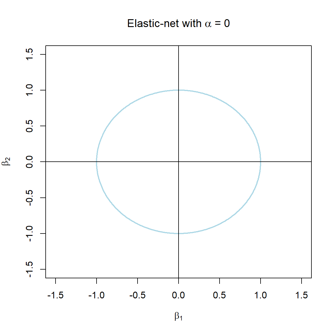
Figure 3.7: The constraint function of elastic-net regularisation for different values of \(\alpha\).

Therefore, there are now two hyperparameters to tune simultaneously, and the choice of \(\alpha\) influences the range of \(\lambda\) values we should consider searching over – compare the x-axis ranges of Figures 3.3 and 3.6. The glmnetUtils package – although with some room for improvement at time of writing – provides a convenient way of doing so.

library(glmnetUtils)

set.seed(1)
elasticnet <- cva.glmnet(lpsa ~ ., train_pros, alpha = seq(0, 1, 0.1))
plot(elasticnet)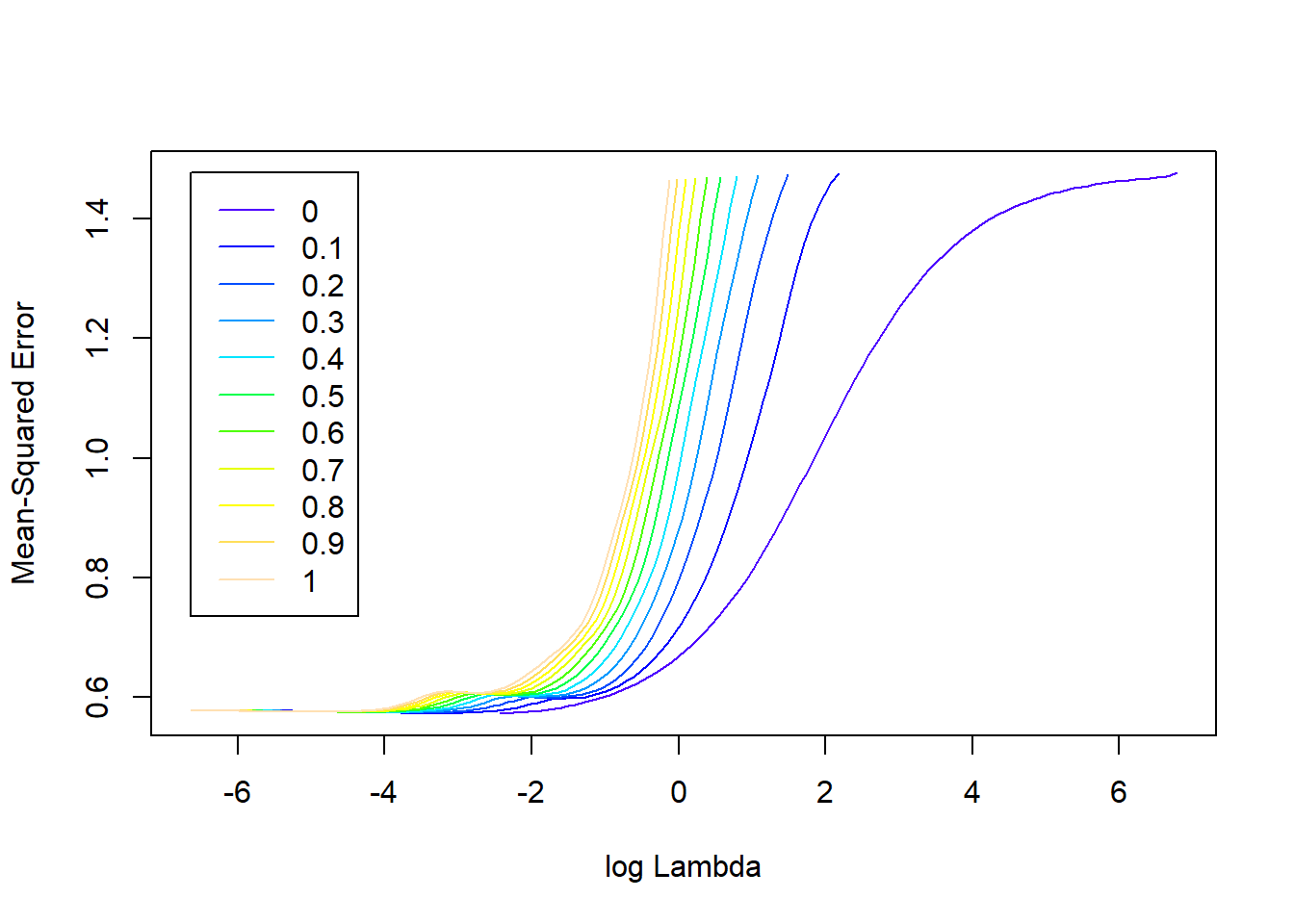

Figure 3.8: Elastic-net regularisation profiles for the prostate cancer dataset.

In Figure 3.8 we see that – for higher values of the regularisation parameter \(\lambda\) – the cross-validated MSE improves as \(\alpha\) decreases, i.e. as \(L_2\) is weighted more. However, if accuracy of prediction is priority, we are interested in the combination of hyperparameters that yields the lowest CV MSE. It is clear that, for this example at least, there is very little difference in the performance of the best models across the different \(\alpha\) values. Regardless, the best combination can be extracted from the resulting model object:

alphas <- elasticnet$alpha #Just extracting the alphas we specified
cv_mses <- sapply(elasticnet$modlist, 
                 function(mod) min(mod$cvm) #Across the list of models, extract the minimum CV MSE
                 )
best_alpha <- alphas[which.min(cv_mses)] #Alpha corresponding to this minumum

It is crucial to reiterate that for this particular example, the difference in CV performance across the \(\alpha\) hyperparameter is close to negligible:

plot(alphas, cv_mses, 'b', lwd = 2, pch = 16, col = 'navy', xlab = expression(alpha), ylab = 'CV MSE',
     ylim = c(0.57, 0.58)) #Scale is crucial, this is still very granular!
abline(v = best_alpha, lty = 3, col = 'red')

Figure 3.9: Minimum CV MSEs across a range of \(\alpha\) values for the prostate cancer dataset.

Nevertheless, the minimum CV MSE is 0.5731454, corresponding to \(\alpha =\) 0, i.e. pure ridge regression. A key consideration for the data scientist is whether this slight improvement in estimated test performance is justified. Earlier, we reasoned that the ridge regularisation penalty corresponding to the minimum CV error does not correspond with the correlation patterns in the data. This emphasises the need to fully interrogate the data, and not just apply these methods in a generic way.

3.4 Homework exercises

1. Show that the penalised RSS for the ridge regression yields \(\hat{\boldsymbol{\beta}} = \left(\boldsymbol{X}'\boldsymbol{X} + \lambda\boldsymbol{I}\right)^{-1}\boldsymbol{X}\boldsymbol{y}\).

---

3. In this context, statisticians often prefer the term co-variates.↩︎

4. Also called the Euclidean norm, or the length of a vector in Euclidean space.↩︎

5. In other words, the big weights are shrunk more than the small weights, and when rescaling the features the relative sizes of the weights change.↩︎

6. Also referred to as the Manhattan norm/distance.↩︎