Chapter 2 Supervised Learning

This chapter aims to briefly summarise the key aspects of supervised learning that will be relevant for the following sections, some of which you should be familiar with already. Whereas there are many good sources that provide a more comprehensive discussion, Chapter 2 of James et al. (2013) is sufficient for the level and scope of this course.

Using a set of observations to uncover some underlying process in the real world is the basic premise of “learning from data” (Abu-Mostafa et al., 2012, p. 11). By discerning patterns, relationships, and trends within the data, machines become capable of making informed decisions and predictions in various domains. Different learning paradigms have developed to address different problems and data structures, and are generally divided into three broad classes: supervised learning, unsupervised learning, and reinforcement learning. We will not discuss the latter in this course.

The basic distinction is that supervised learning refers to cases where there is some target variable, usually indicated as $Y$, whereas if we are interested in the structures and patterns in explanatory variables¹ only, we refer to unsupervised learning.

Given a quantitative response $Y$ and a set of $p$ predictors $X_1, X_2, \ldots, X_p$, we are interested in the assumed, unobserved function that maps the inputs to the outputs:

\[Y = \underbrace{f(X)}_{systematic} + \underbrace{\epsilon}_{random},\]

where $f(.)$ represents the fixed, but unknown function and $\epsilon$ is a random error term, independent of $X$, with $E(\epsilon) = 0$. By estimating $f$ such that

\[\hat{Y} = \hat{f}(X),\]

we allow for both prediction of $Y$ – which is the primary goal in forecasting – and inference, i.e. describing how $Y$ is affected by changes in $X$.

Hypothesising $\hat{f}$ can be done in two ways, namely via a parametric or a non-parametric approach.

Parametric approach

Here an assumption is made about the functional form of $f$, for example the linear model

\[f(\boldsymbol{X}) = \beta_0 + \sum_{j=1}^p\beta_jX_j.\]

The best estimate of $f$ is now defined as the set of parameters $\hat{\boldsymbol{\beta}}$ that minimise some specified loss function. Given a set of observations $\mathcal{D}=\{\boldsymbol{x}_i, y_i\}_{i=1}^n$ – henceforth referred to as the training set – we could use ordinary least squares to minimise the mean squared error (MSE):

\[MSE = \frac{1}{n}\sum_{i=1}^n\left[y_i - \hat{f}(x_i)\right]^2 \] Therefore, the problem of estimating an arbitrary p-dimensional function is simplified to fitting a set of parameters.

Non-parametric approach

Another option is to make no explicit assumptions regarding the functional form of $f$. This allows one to fit a wide range of possible forms for $f$ – in these notes we consider K-nearest neighbours and tree-based methods – but since estimation is not reduced to estimating a set of parameters, this approach generally requires more data than parametric estimation.

The objective remains to find $f$ that fits the available data as closely as possible, whilst avoiding overfitting to ensure that the model generalises well to unseen data.

Generalisation

The primary goal of prediction is of course to accurately predict the outcomes of observations not yet observed by the model, referred to as out-of-sample observations.

Consider the case where the estimated function $\hat{f}$ is fixed and out-of-sample observations of the variables are introduced, which we will denote as $\{\boldsymbol{x}_0, y_0\}$. The expected MSE for these test set observations (see Section 2.2) can be deconstructed as follows:

\[\begin{align} E\left[y_0 - \hat{f}(\boldsymbol{x}_0) \right]^2 &= E\left[f(\boldsymbol{x}_0) + \epsilon - \hat{f}(\boldsymbol{x}_0)\right]^2 \\ &= E\left[\left(f(\boldsymbol{x}_0) - \hat{f}(\boldsymbol{x}_0)\right)^2 + 2\epsilon \left(f(\boldsymbol{x}_0) - \hat{f}(\boldsymbol{x}_0) \right) + \epsilon^2\right] \\ &= E\left[f(\boldsymbol{x}_0) - \hat{f}(\boldsymbol{x}_0)\right]^2 + 2E[\epsilon]E\left[f(\boldsymbol{x}_0) - \hat{f}(\boldsymbol{x}_0)\right] + E\left[\epsilon^2\right] \\ &= \underbrace{E\left[f(\boldsymbol{x}_0) - \hat{f}(\boldsymbol{x}_0)\right]^2}_{reducible} + \underbrace{Var(\epsilon)}_{irreducible} \tag{2.1} \end{align}\]

The primary goal of machine learning is to find an $\hat{f}$ that best approximates the underlying, unknown relationship between the input and output variables by minimising the reducible error. Note that because of the irreducible component (the “noise” in the data), there will always be some lower bound for the theoretical MSE, and that this bound is almost always unknown in practice (James et al., 2013, p. 19).

In order to achieve accurate out-of-sample prediction, we need to specify a model (another term for the estimated function $\hat{f}$) that is sufficiently – but not overly – complex. Finding this balance of complexity is referred to as the bias-variance trade-off. The reducible error component can be decomposed further to help illustrate this trade-off.

2.1 Bias-variance trade-off

Consider again a fixed $\hat{f}$ and out-of-sample observations $\{\boldsymbol{x}_0, y_0\}$. For ease of notation, let $f = f(\boldsymbol{x}_0)$ and $\hat{f} = \hat{f}(\boldsymbol{x}_0)$. Also note that $f$ is deterministic such that $E\left[f\right] = f$.

Starting with the reducible error in Equation (2.1), we have

\[\begin{align} E\left[f - \hat{f} \right]^2 &= E\left[\hat{f} - f \right]^2 \\ &= E\left[\hat{f} - E(\hat{f}) + E(\hat{f}) - f \right]^2 \\ &= E\left\{ \left[\hat{f} - E(\hat{f})\right]^2 + 2\left[\hat{f} - E(\hat{f})\right] \left[E(\hat{f}) - f\right] + \left[E(\hat{f}) - f\right]^2 \right\} \\ &= E\left[\hat{f} - E(\hat{f})\right]^2 + 2E\left\{\left[\hat{f} - E(\hat{f})\right] \left[E(\hat{f}) - f\right]\right\} + E\left[E(\hat{f}) - f\right]^2 \\ &= Var\left[\hat{f}\right] + 0 + \left[E(\hat{f}) - f\right]^2 \\ &= Var\left[\hat{f}\right] + Bias^2\left[\hat{f}\right] \tag{2.2} \end{align}\]

Showing that the crossproduct term equals zero:

\[\begin{align} E\left\{\left[\hat{f} - E(\hat{f})\right] \left[E(\hat{f}) - f\right]\right\} &= E\left[\hat{f}E(\hat{f}) - E(\hat{f})E(\hat{f}) - \hat{f}f + E(\hat{f})f\right] \\ &= E(\hat{f})E(\hat{f}) - E(\hat{f})E(\hat{f}) - E(\hat{f})f + E(\hat{f})f \\ &= 0 \end{align}\]

Therefore, in order to minimise the expected test MSE we need to find a model that has the lowest combined variance and (squared) bias.

The variance represents the extent to which $\hat{f}$ changes between different randomly selected training samples taken from the same population. The bias of $\hat{f}$ is simply the error that is introduced by approximating the real-world relationship with a simpler representation. Note that since $f$ is generally unknown, the bias component cannot be directly observed or measured outside of simulations. However, these simulations may help us illustrate how the bias and variance change as model complexity increases.

Although the concepts of model complexity and flexibility are not necessarily perfectly defined – depending on the class of model being hypothesised – the following example should provide an intuitive understanding.

2.1.1 Example 1 – Simulation

To allow for easy visualisation, let us consider a simple function with only one feature:

\[Y = X + 2\cos(5X) + \epsilon,\] where $\epsilon \sim N(0, 2)$.

Below we simulate $n = 100$ observations from $X \sim U(-2,2)$, to which we fit cubic smoothing splines of increasing complexity. The details of splines are beyond the scope of this course, but they provide an easy-to-see illustration of “flexibility”.

rm(list = ls())
set.seed(4026)

#Simulated data
n <- 100
x <- runif(n, -2, 2)
y <- x + 2*cos(5*x) + rnorm(n, sd = sqrt(2))

#The true function
xx <- seq(-2, 2, length.out = 1000)
f <- xx + 2*cos(5*xx)

#Fit cubic splines with increasing degrees of freedom
for(dof in 2:50){
  fhat <- smooth.spline(x, y, df = dof)
  plot(x, y, pch = 16)
  lines(xx, f, 'l', lwd = 2)
  lines(fhat, col = 'blue', lwd = 2)
  title(main = paste('Degrees of freedom:', dof))
  legend('bottomright', c('f(x) - True', expression(hat(f)(x) ~ '- Cubic spline')), 
         col = c('black', 'blue'), lty = 1, lwd = 2)
}

$Cubic splines with varying degrees of freedom fitted to a sample of 100 datapoints drawn from $Y = X + 2\cos(5X) + \epsilon$, with $\epsilon \sim N(0, 2)$.$

Figure 2.1: Cubic splines with varying degrees of freedom fitted to a sample of 100 datapoints drawn from $Y = X + 2\cos(5X) + \epsilon$, with $\epsilon \sim N(0, 2)$.

This serves to illustrate how the model’s degrees of freedom are directly proportional to the model’s complexity. However, to extricate the bias and variance components, we need to observe these models’ fit on out-of-sample data across many random realisations of training samples.

In the following simulation we again observe $n=100$ training observations at a time, to which the same models of varying complexity as above are fitted. Each model’s fit is then assessed on a set of 100 testing observations, where the $\boldsymbol{x}_0$ (and, therefore, true $f(\boldsymbol{x}_0)$) are fixed, but random noise is added. This process is repeated 1000 times, such that we can keep track of how each test observation’s predictions vary across the iterations, as well as the errors.

set.seed(1)

n <- 100          #Sample size
num_sims <- 1000  #Number of iterations (could be parallelised)
dofs <- 2:25      #Model complexities
var_eps <- 2      #Var(epsilon): The irreducible error

pred_mat <- matrix(nrow = num_sims, ncol = n) #To store each set of predictions
mses <- vector(length = num_sims)             #Also want to track the testing MSEs
red_err <- vector(length = num_sims)          #As well as the reducible error

#Herein we will capture the deconstructed components for each model
results <- data.frame(Var = NA, Bias2 = NA, Red_err = NA, MSE = NA)

#Testing data
x_test <- runif(n, -2, 2)
f_test <- x_test + 2*cos(5*x_test) #This is the part we don't know outside sims!!

d <- 0 #To keep track of dof iterations, even when changing the range

for(dof in dofs) { #Repeat over all model complexities
  d <- d+1
  for(iter in 1:num_sims){ 
    
    #Training data
    x_train <- runif(n, -2, 2)
    y_train <- x_train + 2*cos(5*x_train) + rnorm(n, sd = sqrt(var_eps))
    
    #Add the noise
    y_test <- f_test + rnorm(n, sd = sqrt(var_eps))
    
    #Fit cubic spline
    spline_mod <- smooth.spline(x_train, y_train, df = dof)
    
    #Predict on OOS data
    yhat <- predict(spline_mod, x_test)$y
    
    #And store
    pred_mat[iter, ] <- yhat
    red_err[iter] <- mean((f_test - yhat)^2)
    mses[iter] <- mean((y_test - yhat)^2)
  }
  
  #Average each component over all iterations
  var_fhat <- mean(apply(pred_mat, 2, var))           #E[\hat{f} - E(\hat{f})]^2
  bias2_fhat <- mean((colMeans(pred_mat) - f_test)^2) #E[E(\hat{f}) - f]^2
  reducible <- mean(red_err)                          #E[f - \hat{f}]^2
  MSE <- mean(mses)                                   #E[y_0 - \hat{f}]^2
  
  results[d, ] <- c(var_fhat, bias2_fhat, reducible, MSE)
}

#Plot the results
plot(dofs, results$MSE, 'l', col = 'darkred', lwd = 2,
     xlab = 'Model complexity', ylab = '', ylim = c(0, max(results)))
lines(dofs, results$Bias2, 'l', col = 'lightblue', lwd = 2)
lines(dofs, results$Var, 'l', col = 'orange', lwd = 2)
lines(dofs, results$Red_err, 'l', lty = 2, lwd = 2)
legend('topright', 
       c('MSE', expression(Bias^2 ~ (hat(f))), expression(Var(hat(f))), 'Reducible Error'), 
       col = c('darkred', 'lightblue', 'orange', 'black'), lty = c(rep(1, 3), 2), lwd = 2)

abline(v = dofs[which.min(results$MSE)], lty = 3) #Complexity minimising MSE
abline(h = var_eps, lty = 3)                      #MSE lower bound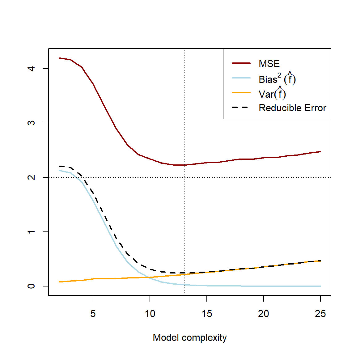

Averaged error components over 1000 simulations of samples of $n=100$. The horizontal dashed line represents the minimum lower bound for the test MSE. The vertical dashed line indicates the point at which both the test MSE and reducible error are minimised.

Figure 2.2: Averaged error components over 1000 simulations of samples of $n=100$. The horizontal dashed line represents the minimum lower bound for the test MSE. The vertical dashed line indicates the point at which both the test MSE and reducible error are minimised.

As a quick sanity check before interpreting this result, let us add up the components – which were calculated separately – and see whether we indeed observe that $E\left[f - \hat{f} \right]^2 = Var\left[\hat{f}\right] + Bias^2\left[\hat{f}\right]$ as per Equation (2.1), and $\text{Test MSE} = E\left[y_0 - \hat{f}\right]^2 = E\left[f - \hat{f} \right]^2 + Var(\epsilon)$ as per Equation (2.2). Note that we will need to have a small tolerance for discrepancy, since we have approximated the expected values by averaging over only 1000 realisations. This approximation will become more accurate as the number of iterations is increased.

#Is reducible error = var(fhat) + bias^2(fhat)?
ifelse(isTRUE(all.equal(results$Red_err, 
                        results$Var + results$Bias2, 
                        tolerance = 0.001)),
       'Happy days! :D', 
       'Haibo...')

## [1] "Happy days! :D"

#Is Test MSE = var(fhat) + bias^2(fhat) + var(eps)?
ifelse(isTRUE(all.equal(results$MSE, 
                        results$Var + results$Bias2 + var_eps, 
                        tolerance = 0.01)),
       'Happy days! :D', 
       'Haibo...')

## [1] "Happy days! :D"

Figure 2.2 illustrates the general error pattern when learning from data: As model complexity/flexibility increases, the variance across multiple training samples increases, whilst the (squared) bias decreases as the estimated function gets closer to the true pattern on average. Note that $E(\epsilon^2) = Var(\epsilon)$ remains constant. This decrease in bias$^2$ initially offsets the increase in variance such that the test MSE initially decreases. However, from some complexity/flexibility of $\hat{f}$, the decrease in bias$^2\left(\hat{f}\right)$ is offset by the increase in $Var\left(\hat{f}\right)$, at which point the model starts to overfit and the test MSE starts increasing. This is the bias-variance trade-off. In this particular example, we see that of all the cubic splines, one with 13 degrees of freedom most closely captures the underlying pattern in the data, as measured by the test MSE.

The fundamental challenge in statistical learning is to postulate a model of the data that yields both a low bias and variance, whilst policing the model complexity such that the sum of these error components are minimised.

In the above example, we knew what the underlying function was as well as the residual variance. However, when modelling data generated in some real-world environment, we do not observe $f$ and therefore cannot explicitly compute the test MSE. In order to estimate the test MSE, we make use of model validation procedures.

2.2 Model validation

Imagine there are two students who have been subjected to the same set of lectures, notes, and homework exercises, which you can view as their training data used to learn the true subject knowledge. When studying for the test – which is designed to test this knowledge, i.e. the test set in our analogy – they take two different approaches: Student A, a model student, tries to master the subject matter by focusing on the course material, testing themself with new homework exercises after studying some completed ones first. Student B, however, managed to obtain a copy of the test in advance through some nefarious means, and plans to prove their knowledge of the subject matter by preparing only for this specific set of questions.

Even though student B’s test score will in all likelihood be better, does this mean that they have obtained and retained more knowledge? Certainly not! Suppose the lecturer catches wind of this cheating and swaps the initial test with a new set of randomised questions. Which of the two approaches would you expect to yield better results on such a test, on average?

When comparing different statistical models, we would like to select the one that we think will work best on unseen test data. But if we use the test data to make this decision, this will also be cheating, and we will be no better off for it. Like student A though, we can leave out some exercises in the training data and use these to validate our learning, i.e. gauge how well we would do in the test.

2.2.1 Validation set

One way to create a validation set (or hold-out set) is to just leave aside, in a randomised way, a portion of the training data, say 30%. We then train models on the other 70% of the data only, test them on the validation set, and select the model that yields the lowest validation MSE, which serves as an estimate of test set performance.

Although there are some situations in which this approach is merited, it has two potential flaws:

Due to the single random split, the validation estimate of the test error can be highly variable.
Since we are reducing our training data, the model sees less information, generally leading to worse performance. Therefore, the validation error may overestimate the test error.

We will not go into any more detail than this on the validation set approach, but rather focus on cross-validation (CV) strategies, which addresses these two issues.

2.2.2 $k$-fold CV

With this approach, the training set is randomly divided into $k$ groups, or folds, of (approximately) the same size. Each fold gets a turn to act as the validation set, with the model trained on the remaining $k-1$ folds. Therefore, the training process is repeated $k$ times, each yielding an estimate of the test error, denoted as $MSE_1,\ MSE_2,\ldots,\ MSE_k$. These values are then averaged over all $k$ folds to yield the $k$-fold CV estimate:

\[CV_{(k)} = \frac{1}{k}\sum_{i=1}^k MSE_i\] The next obvious question is: What value of $k$ should we choose? Start by considering the lowest value, $k=2$. This would be the same as the validation set approach with a 50% split, except that each half of the data will get a chance to act as training and validation set. Therefore, we still expect the validation error to overestimate the test error, or in other words, there will be some bias. As we increase $k$, the estimated error will become more unbiased, since each fold will allow the model to capture more of the underlying pattern.

However, just as with model complexity we also need to consider the variance aspect. Consider now the other extreme, when $k = n$ (the number of observations in the training set). Here we have what is referred to as Leave-one-out cross-validation (LOOCV), since we have $n$ folds, each leaving out just one observation for validation. Each of these $n$ training sets will be almost identical, such that there will be very high correlation between them. Now, remember that when we add correlated random variables (note that averaging involves summation), then the correlation affects the resulting variance:

\[Var(X+Y) = \sigma^2_X + \sigma^2_Y + 2\frac{\rho_{XY}}{\sigma_X\sigma_Y}\] Therefore, larger $k$ implies larger variation of the estimated error. This means that the same bias-variance trade-off applies to $k$-fold CV! In practice, it has been shown that $k = 5$ or $k = 10$ yields a good balance such that the test error estimate does not suffer from excessively high bias nor variance.

Also note that as $k$ increases, the computational cost increases proportionally, since $k$ separate models must be fitted to $k$ different data splits. This could cause unnecessarily long training times for large datasets/complicated models, such that a smaller $k$ might be preferable.

To illustrate the implementation, let us return to the earlier example, where we will pretend that we do not know the underlying relationship we are trying to estimate.

2.2.3 Example 1 – Simulation (continued)

Before using the CV error to determine the ideal model complexity, let us first illustrate the concept of cross-validation for a single model, say a cubic spline with 8 degrees of freedom, with $k = 10$.

set.seed(4026)

#Simulated data
n <- 100 
k <- 10  #We will apply 10-fold CV
x <- runif(n, -2, 2)
y <- x + 2*cos(5*x) + rnorm(n, sd = sqrt(2))

#Here we will collect the out-of-sample and in-sample errors
cv_k <- c()
train_err <- c()

# We don't actually need to randomise, since x's are random, but one should in general
ind <- sample(n) 
x <- x[ind]
y <- y[ind]

folds <- cut(1:n, breaks = k, labels = F)   #Create indices for k folds

#10-fold CV
for(fld in 1:k){
  x_train <- x[folds != fld]                    #Could streamline this code, (see next block)
  x_valid <- x[folds == fld]                    #but this is easier to follow   
  y_train <- y[folds != fld]                    
  y_valid <- y[folds == fld]
  fit <- smooth.spline(x_train, y_train, df = 8)
  valid_pred <- predict(fit, x_valid)$y
  train_pred <- predict(fit, x_train)$y
  cv_k <- c(cv_k, mean((valid_pred - y_valid)^2))
  train_err <- c(train_err, mean((train_pred - y_train)^2))
  
  #One should rather write the above into a function... 
  #But the plotting needs to be inside the loop for the notes' rendering
  par(mfrow = c(1, 2))
  plot(x_train, y_train, pch = 16, xlab = 'x', ylab = 'y', 
       xlim = c(min(x), max(x)), ylim = c(min(y), max(y)))
  points(x_valid, y_valid, pch = 16, col = 'gray')
  segments(x_valid, y_valid, x_valid, valid_pred,
           col = 'red', lty = 3, lwd = 2)
  lines(fit, col = 'blue', lwd = 2)
  title(main = paste('Fold:', fld))
  legend('bottomright', c('Training', 'Validation', 'Errors'), 
         col = c('black', 'gray', 'red'), 
         pch = c(16, 16, NA),
         lty = c(NA, NA, 3),
         lwd = c(NA, NA, 2))
  plot(1:fld, cv_k, 'b', pch = 16, col = 'red', lwd = 2, xlab = 'Fold', ylab = 'MSE', 
       xlim = c(1, 10), ylim = c(1, 5.5))
  lines(1:fld, train_err, 'b', pch = 16, lwd = 2)
  legend('topright', c('Training', 'Validation'), col = c('black', 'red'), lwd = 2)
}

Left: The training (black) and validation (grey) portions of the dataset across 10 folds, with the fitted cubic spline with 8 degrees of freedom in blue. Right: The resulting training (black) and validation (red) MSEs across 10 folds.

Figure 2.3: Left: The training (black) and validation (grey) portions of the dataset across 10 folds, with the fitted cubic spline with 8 degrees of freedom in blue. Right: The resulting training (black) and validation (red) MSEs across 10 folds.

Here we see that, as expected, the validation error is noticeably more variable than the training error across the folds. We can calculate² the CV MSE as 2.77, although on its own this value is not particularly insightful. When comparing it to that of other models, though, we can determine which model complexity is estimated to yield the lowest test error.

#Keep track of MSE per fold, per model
fold_mses <- matrix(nrow = 10, ncol = length(dofs))

for(fld in 1:k){
  d <- 0
  for(dof in dofs){ #Using the same dofs as earlier
    d <- d + 1
    fit <- smooth.spline(x[folds != fld], y[folds != fld], df = dof) 
    valid_pred <- predict(fit, x[folds == fld])$y
    fold_mses[fld, d] <- mean((valid_pred - y[folds == fld])^2)
  }
}
#Average over all folds
cv_mses <- colMeans(fold_mses)

# Compare the true MSE from earlier
plot(dofs, results$MSE, 'l', col = 'darkred', lwd = 2,
     xlab = 'Model complexity', ylab = '', ylim = c(0, max(cv_mses)))
lines(dofs, cv_mses, 'l', col = 'grey', lwd = 2)
legend('bottomright', c('CV MSE', 'True test MSE'), col = c('gray', 'darkred'), lty = 1, lwd = 2)
abline(v = dofs[which.min(results$MSE)], lty = 3)
points(dofs[which.min(cv_mses)], min(cv_mses), pch = 13, cex = 2.5, lwd = 2)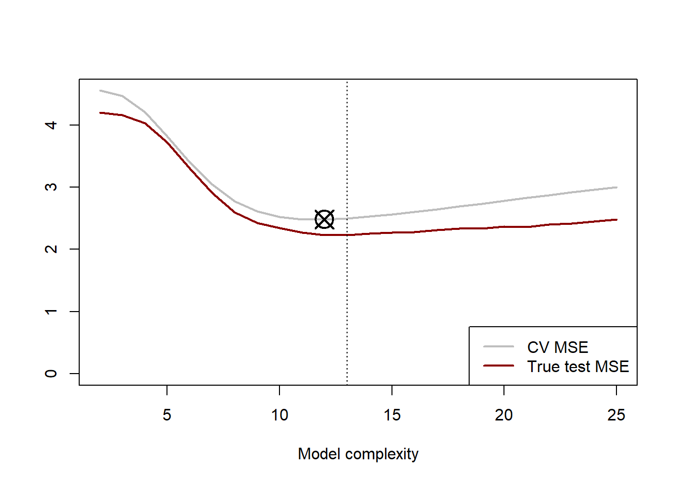

10-fold cross-validation error curve (grey) for cubic splines with varying degrees of freedom, with the minimum point indicated by the crossed circle. The red line indicates the true test MSE being estimated.

Figure 2.4: 10-fold cross-validation error curve (grey) for cubic splines with varying degrees of freedom, with the minimum point indicated by the crossed circle. The red line indicates the true test MSE being estimated.

Because we simulated these data, we know that the cubic spline yielding the lowest expected test MSE is one with 13 degrees of freedom. Applying 10-fold CV to our 100 training data points resulted in an estimated optimal model with 12 degrees of freedom, indicated by the crossed square in Figure 2.4. It is interesting to note that the CV error consistently overestimated the true error. This is likely due to the relatively small dataset; remember that we only tested on 10 observations per fold! The shape of the true MSE curve was captured relatively well by the CV process in this example.

This section provided a succinct illustration of model validation. For a detailed discussion, see Section 5.1 of James et al. (2013). In the following chapters we will move beyond simulated data and apply these methods to various datasets as we encounter different classes of models and other techniques. Although there is much value in coding the CV procedure from scratch, it is built into various R packages, which we will leverage going forward.

2.3 Side note: Statistical learning vs machine learning

It may seem that we use the terms “statistical learning” and “machine learning” interchangeably, so is there a difference? The distinction between these two concepts can sometimes be blurred with the paradigms largely overlapping, and some might argue that the difference is mostly semantic.

In essence, statistical learning often focuses on understanding the probabilistic relationships between variables, while machine learning places greater emphasis on developing algorithms that can learn patterns directly from data, sometimes sacrificing interpretability for predictive performance. However, the principles discussed in this chapter form the core of both approaches – both are concerned with extracting insights from data and making predictions, although they may approach these goals with slightly different philosophical and methodological perspectives.

Statistical learning places a strong emphasis on understanding the underlying data-generating process and making inferences about population characteristics based on sample data. While understanding the underlying data-generating process is still important in machine learning, the focus is often more on achieving optimal predictive performance. Statistical learning approaches are also characterised by explicit assumptions about the underlying statistical distributions and relationships between variables, whereas machine learning methods often work in a more agnostic manner and may not rely heavily on explicit statistical assumptions.

For the purposes of our study throughout this course, these distinctions are not of consequence and we will adopt both perspectives throughout.

2.4 Homework exercises

For Example 1, edit the provided code such that LOOCV is applied. Does this method suggest a different model complexity?
Now do the same for 5-fold CV. What changes in the CV curve do you observe as $k$ changes?

Often referred to as features in the learning context, or predictors in supervised learning specifically.↩︎
Since there were 100 observations and 10 folds, each fold had an equal number of observations and we can calculate the CV MSE as the average of the 10 folds’ average errors. However, in cases where there are unequal numbers of observations across the folds, it would be more accurate to average over all of the individual observations’ squared errors.↩︎

STA4026S – Honours Analytics
Section A: Theory and Application of Supervised Learning