Chapter 6 Tree-based Methods
The final topic in this section of the course is tree-based methods, i.e. decision trees10 and their extensions. We will cover classification and regression trees, random forests, and gradient boosted trees. Although chapter 8 of James et al. (2013) contains a concise summary of these methods, the interested reader is rather referred to section 9.2 of Hastie et al. (2009) for trees and chapter 15 for random forests, and section 16.4 of Murphy (2013) for boosting.
Classification and regression trees – often abbreviated as CART or just referred to as decision trees collectively – are simple, non-parametric classification/regression methods that utilise a tree structure to model the relationships among the features and the potential outcomes. Although decision trees are conceptually very simple, they can be quite powerful, especially when ensembled. They are built using a heuristic called recursive binary partitioning (divide and conquer) that partitions the feature space into a set of (hyper) rectangles. The prediction following the partitioning depends on whether the response is quantitative on qualitative, hence we will again consider regression and classification problems separately, starting with the former.
6.1 Regression trees
Let \(Y\) denote a continuous outcome variable and let \(X_1, X_2, \ldots, X_p\) be a set of predictors/features, of which we have \(n\) observations. The regression tree algorithm entails repeatedly splitting the p-dimensional feature space into distinct, non-overlapping regions, with the splits orthogonal to the axes.
Suppose that we partition the feature space into \(M\) regions, \(R_1 , R_2, \ldots, R_M\). Then for each region we model the response as a constant, \(c_m\):
\[\begin{equation} f(\boldsymbol{x}) = \sum_{m=1}^Mc_mI(\boldsymbol{x} \in R_m). \tag{6.1} \end{equation}\]As with other regression models, our goal is still to minimise
\[\begin{equation} RSS = \sum_{m=1}^{M}\sum_{i:x_i\in R_m}\left[y_i - \hat{f}(\boldsymbol{x} _i)\right]^2. \tag{6.2} \end{equation}\]Therefore, the best \(\hat{c}_m\) to minimise this criterion is simply the average of the \(y_i\) in each region \(R_j\):
\[\begin{equation} \hat{c}_m = \text{ave}(y_i|\boldsymbol{x}_i \in R_m) \tag{6.3} \end{equation}\]Exhaustively searching over every possible combination of regions is computationally infeasible. Therefore, we use a top-down, greedy algorithm called recursive binary splitting:
First, select the predictor \(X_j\) and split point \(s\) such that the regions \(R_1(j, s) = \{X|X_j < s\}\) and \(R_2(j, s) = \{X|X_j \geq s\}\) lead to the greatest possible reduction in RSS. That is, we consider all predictors \(X_1, \ldots, X_p\), and all possible values of the split point \(s\) for each of the predictors, and then choose the predictor and split point such that Equation (6.2) is minimised.
Next, identify the predictor and split point that best splits one of the previously identified regions, such that there are now three regions.
Continue splitting the regions until a stopping criterion is reached. For instance, we may continue until no region contains more than 5 observations, or when the proportional reduction in \(RSS\) is less than some threshold.
Once the regions \(R_1 , R_2, \ldots, R_M\) have been created, we predict the response for a given test observation using the mean of the training observations in the region to which that test observation belongs.
As a brief side note, the model from Equation (6.1) can also be written in the form
\[f(\boldsymbol{x}) = \sum_{m=1}^Mc_mI(\boldsymbol{x} \in R_m) = \sum_{m=1}^Mc_m \phi(\boldsymbol{x}; \boldsymbol{v}_m),\] where \(\boldsymbol{v}_m\) encodes the choice of variable to split on \((X_j)\) and the split point value \((s)\) on the path from the start (root) to the \(m\)th region (leaf). When viewed as such, a CART model is just an adaptive basis function model (alluded to in the previous chapter), where the basis functions define the regions, and the weights specify the response value in each region (Murphy, 2013, p. 544).
One of the advantages of a decision tree is its visual representation which makes for easy interpretation. This is best illustrating via an example.
6.1.1 Example 6 – California housing
In this example we consider a well-known dataset from the 1990 California census, which contains aggregated data for 20 640 neighbourhoods. The variables include information like the neighbourhood’s median house age, the median income, total number of bedrooms and bathrooms, number of households, population, and the location, as can be seen here:
library(DT)
calif <- read.csv('data/calif.csv')
datatable(calif, options = list(scrollX = T, pageLength = 6))
For now, we will only use the spatial information (latitude and longitude) to model the target variable: (log of) median house price.
We begin by plotting a map of the data – a 2-dimensional feature space – using a colour scale to indicate the target variable.
library(maps)
library(RColorBrewer) # For colourblind friendly palettes

# Replace with log
calif$HousePrice <- log(calif$HousePrice)

# Make custom colour scale
n_breaks <- 9
my_cols <- brewer.pal(n_breaks, 'YlOrBr')[cut(calif$HousePrice, breaks = n_breaks)]

# Plot the data
plot(calif$Longitude, calif$Latitude, pch = 16, cex = 0.5, bty = 'L',
     xlab = 'Longitude', ylab = 'Latitude', col = my_cols)
legend(x = 'topright', bty = 'n', title = 'Log Median House Price', cex = 0.9,
       legend = round(seq(min(calif$HousePrice), max(calif$HousePrice), length.out = n_breaks), 2),
       fill = brewer.pal(n_breaks, 'YlOrBr'))

# Add the state border
par(new = TRUE)
map('state', 'california', add = T, lwd = 2) |> invisible()
text(-123, 35, 'Pacific Ocean')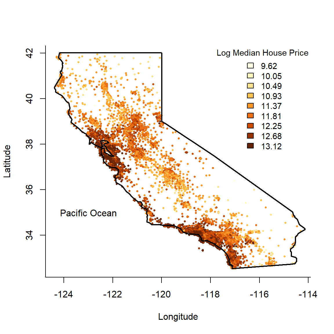
Figure 6.1: Californian median neighbourhood house prices (logscale) in 1990.
We can now proceed to partition the feature space using recursive binary splitting, resulting in a regression tree. There are many packages in R that implement decision trees. We will be using one of the more basic ones: tree. For now we are not going to split into training and testing; for illustrative purposes we shall use the entire dataset.
Using the default stopping criteria, we fit the following decision tree shown below in Figure 6.2
library(tree)

#Easy as one, two, tree
calif_tree <- tree(HousePrice ~ Latitude + Longitude, data = calif)

# Plot the tree
plot(calif_tree)
text(calif_tree)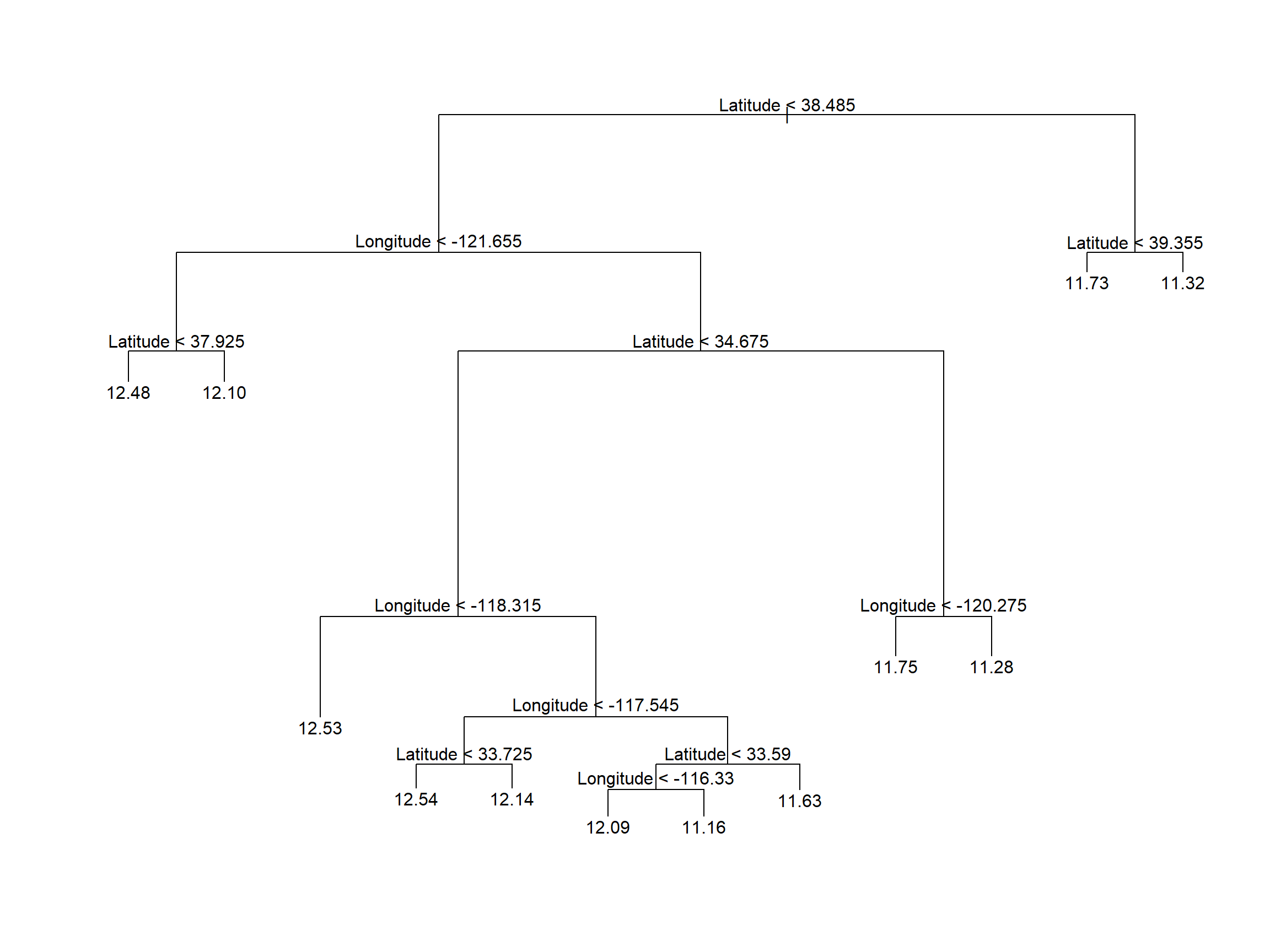
Figure 6.2: Vanilla regression tree fitted to the Cailfornia dataset
The corresponding feature space is shown below in Figure 6.3.
# Plot the data again
plot(calif$Longitude, calif$Latitude, pch = 16, cex = 0.5,
     col = my_cols, xlab = 'Longitude', ylab = 'Latitude', bty = 'o')

# And add the partitioned feature space
partition.tree(calif_tree, ordvars = c('Longitude', 'Latitude'), add = T, lwd = 3)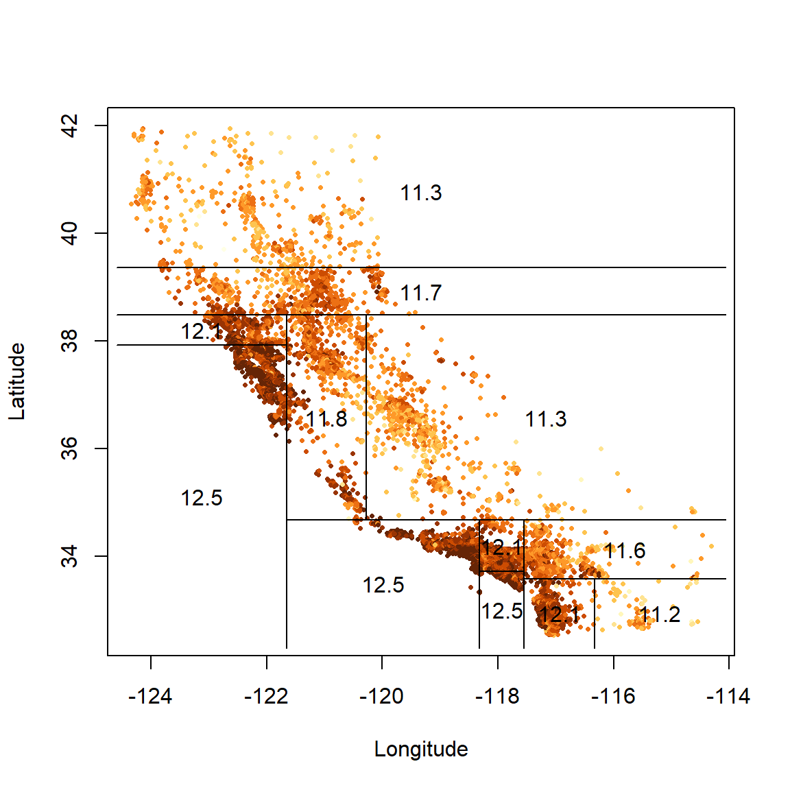
Figure 6.3: Partitioned feature space for vanilla regression tree fitted to the Cailfornia dataset
The labels in Figure 6.2 indicate both the splitting variable and the split point. All data points below the split point for that variable go to the left of that branch or, equivalently, are left/below the resulting line in the partitioned feature space.
The final regions correspond to the ends of the tree’s branches, which are indeed referred to as leaves, or terminal nodes. The leaf values are the fitted values for all the data points in that region, which is just the average (Equation (6.3)).
It is easy to see visually that the algorithm attempts to group together pockets of most-similar observations. Again, though, the question arises of when to stop? This returns us to the same consideration we encountered in all previous models, namely that of model complexity.
6.1.2 Cost complexity pruning
A decision tree’s complexity is measured by the number of leaves (which is equal to the number of splits + 1). We could continue splitting until every single observation is in its own region, such that the training \(RSS = 0\) (each \(y_i\) will be equal to its region’s average). However, this would be extreme overfitting, and the model would perform very poorly on unseen data. As with all statistical learning algorithms, we need to determine the ideal level of complexity that captures as much information as possible without overfitting.
One way of controlling complexity is to continue growing the tree only until the decrease in RSS fails to exceed some high threshold. However, this is short-sighted since a split later on might produce an even greater reduction in RSS. A better strategy is therefore to grow a very large tree and then prune it back to obtain a smaller subtree.
Since our goal is to find the subtree with the lowest test error, we can estimate any given subtree’s test error using cross-validation. However, estimating the CV error for every possible subtree is not computationally feasible. Instead we only consider a sequence of trees obtained by pruning the full tree back in a nested manner. This tree pruning technique is known as cost complexity pruning, or weakest link pruning, and is essentially a form of regularisation.
Let \(T_0\) be the full tree and let \(T\subseteq T_0\) be a subtree with \(|T|\) terminal nodes or, equivalently, regions in the feature space. We now penalise the RSS according to \(|T|\):
\[\begin{equation} RSS_{\alpha} = \sum_{m=1}^{|T|}\sum_{i:x_i\in R_m}\left[y_i - \hat{f}(\boldsymbol{x} _i)\right]^2 + \alpha|T|, \tag{6.4} \end{equation}\]where \(\alpha \ge 0\) is a tuning parameter.
When \(\alpha = 0\), \(RSS_{\alpha} = RSS\) and therefore \(T=T_0\). For values of \(\alpha > 0\), we seek the subtree \(T\) that minimises \(RSS_{\alpha}\). As \(\alpha\) increases, subtrees with a large number of leaves are penalised more heavily and a smaller \(T\) will be favoured such that branches are “pruned” off. This happens in a nested fashion, such that we can easily obtain subtrees as a function of \(\alpha\).
By choosing \(\alpha\), we are effectively selecting a subtree; that is, a more parsimonious model that does not overfit the sample data. We want the subtree (and hence \(\alpha\) value) that has the lowest test error and therefore has the best predictive performance on unseen data. Therefore, we will once again use CV to determine this \(\alpha\)/subtree.
To illustrate this, we return to the California dataset, this time using all the predictors.
# First fit larger tree by relaxing stopping criteria
# ?tree.control
# minsize: will only consider split if at least so many observations in node
# mincut: will only split if both child nodes then have at least so many
# mindev: will only consider split if within-node deviance is at least this times root RSS

stopcrit <- tree.control(nobs = nrow(calif), mindev = 0.003)
calif_bigtree <- tree(HousePrice ~ . , data = calif, control = stopcrit)
(s <- summary(calif_bigtree))
##
## Regression tree:
## tree(formula = HousePrice ~ ., data = calif, control = stopcrit)
## Variables actually used in tree construction:
## [1] "Income" "Latitude" "Longitude" "HouseAge"
## Number of terminal nodes: 25
## Residual mean deviance: 0.1162 = 2396 / 20620
## Distribution of residuals:
## Min. 1st Qu. Median Mean 3rd Qu. Max.
## -2.86000 -0.21050 -0.01136 0.00000 0.19030 2.03900By slightly relaxing the stopping criterion of RSS reduction, we increased the size of the tree to 25. We also see that the only features used to split were income, house age, and latitude and longitude, so the location information was indeed very useful!
Plotting the tree at this size is already quite messy (Figure 6.4), with a lot of unnecessary, indistinguishable information at the bottom.
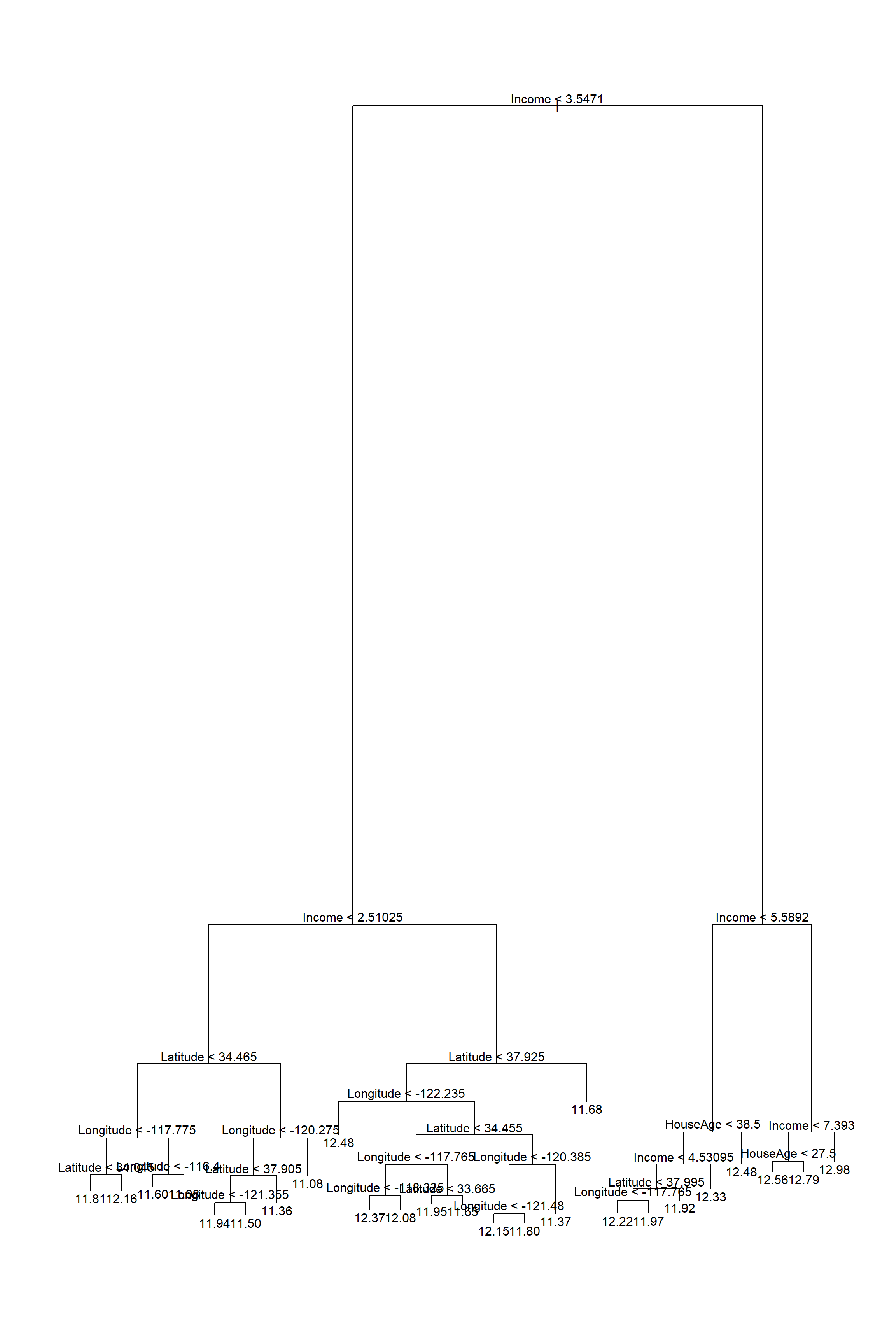
Figure 6.4: Large regression tree fitted to the Cailfornia dataset
We now apply cost complexity pruning, measuring the CV RSS for each subtree.
set.seed(4026)
calif_cv <- cv.tree(calif_bigtree)

# See str(calif_cv)
# size = number of terminal nodes
# dev = RSS
# k = alpha (tuning parameter that determines tree size)

calif_cv$k[1] <- 0 #First entry was -Inf

# Plot everything
plot(calif_cv$size, calif_cv$dev, type = 'o',
     pch = 16, col = 'navy', lwd = 2,
     xlab = 'Number of terminal nodes', ylab = 'CV RSS')
axis(side = 1, at = 1:max(calif_cv$size), labels = 1:max(calif_cv$size))

# Add alpha values to the plot:
alpha <- round(calif_cv$k)
axis(3, at = calif_cv$size, lab = alpha)
mtext(expression(alpha), 3, line = 2.5, cex = 1.5)

# Highlight the minimum CV Error
T <- calif_cv$size[which.min(calif_cv$dev)]
abline(v = T, lty = 2, lwd = 2, col = 'red')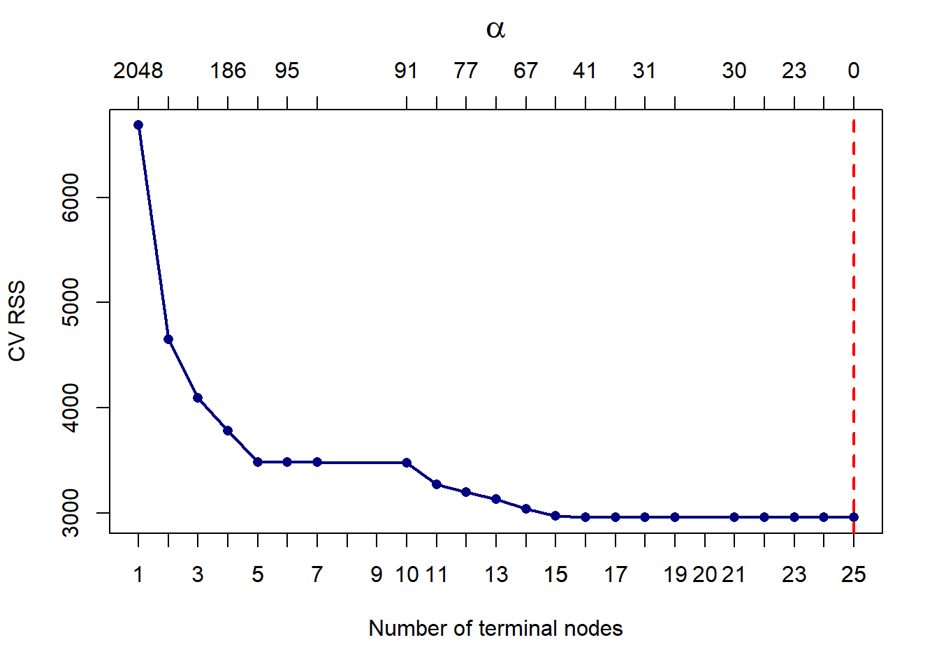
Figure 6.5: Cross-validated pruning results on the large tree fitted to the Cailfornia dataset
We can see that the CV error did indeed keep decreasing. To check this, we show that the minimum RSS is indeed observed at 25 terminal nodes:
## [1] 25However, the improvement in results is negligible from about 15 leaves. One could certainly also argue that a tree of size 5 might be preferable, given that it performs comparably to a tree of size 10, and the improvement from that point on is not drastic. In fact, decision trees will rarely be used for prediction purposes, since they will most often be outperformed by other algorithms. Their main value arguably lies in their interpretability, hence we will consider opting for the simpler model.
# Prune the tree
calif_pruned5 <- prune.tree(calif_bigtree, best = 5)
plot(calif_pruned5)
text(calif_pruned5)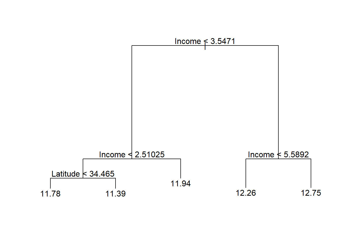
Figure 6.6: Cailfornia housing regression tree pruned to 5 terminal nodes
We see that this tree only uses income and latitude as splitting variables, perhaps suggesting that it is too simplistic, especially when compared to the 15-node tree. In Figure 6.7 we see that although the gain in RSS reduction is comparatively limited, the later splits make extensive use of the location information. However, for neighbourhoods with a median income above 3.547, only income and house age were used in subsequent splits, indicating less interaction between income and location in the wealthy areas.
# Prune the tree
calif_pruned15 <- prune.tree(calif_bigtree, best = 15)
plot(calif_pruned15)
text(calif_pruned15)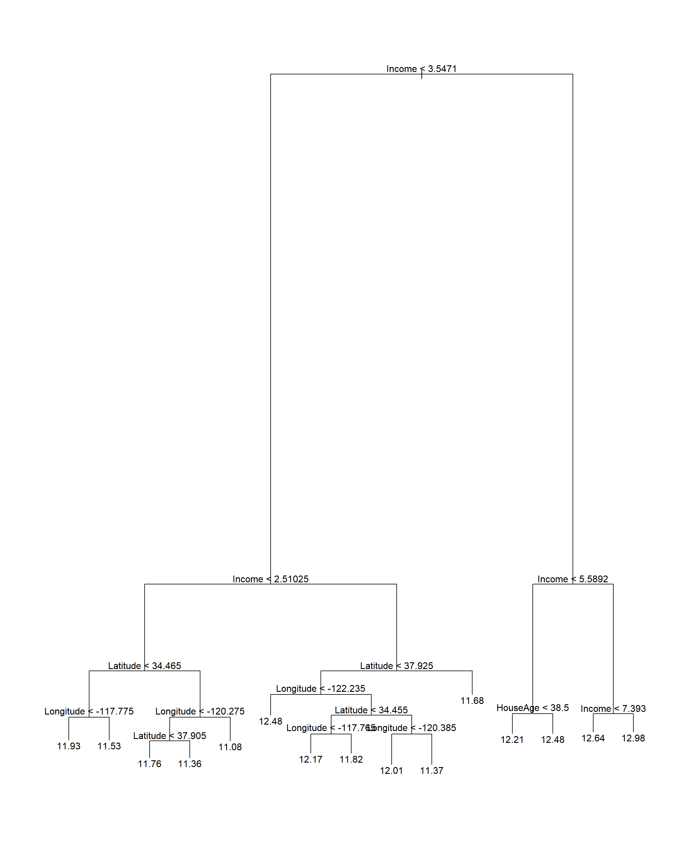
Figure 6.7: Cailfornia housing regression tree pruned to 15 terminal nodes
This example primarily serves to illustrate the interpretive properties of decision trees. We will explore their sensitivity to sampling variation and their performance on unseen data later once ensembling methods are introduced. First, however, we will see how this method can be used to classify a qualitative response.
6.2 Classification trees
Consider now a categorical response variable \(Y \in \{1, 2, \ldots, K\}\). Just like with regression trees, classification trees split the feature space into \(M\) regions which correspond to the terminal (leaf) nodes of the tree. In lieu of an average to calculate for the observations falling within each region, the predicted value of an observation with \(X \in R_m\) will now be the most commonly occurring class in \(R_m\).
The class proportions in each terminal node provide an indication of the reliability of the prediction:
\[\begin{equation} \hat{p}_{mk} = \frac{1}{N_m} \sum_{i:x_i\in R_m} I(y_i = k), \tag{6.5} \end{equation}\]where \(N_m\) denotes the number of observations in region \(R_m\).
Although classification trees are also grown by recursive binary splitting, RSS cannot be used as splitting criterion. Now, we could grow the tree by choosing the split that minimises the classification error at each step, i.e. minimise the proportion of incorrectly predicted observations. In practice, however, splitting on the reduction in classification error does not produce good trees. We will instead consider the following three splitting criteria, all of which are designed to measure node impurity.
6.2.1 Splitting criteria
We would like the leaf nodes to be as homogeneous or “pure” as possible, with each leaf node ideally containing observations of only one response category. When deciding where to split on a particular dimension, we can use the following measurements to measure the resulting homogeneity.
1. Gini Index
Arguably the simplest way of measuring node impurity is via the Gini index (also referred to as Gini impurity or Gini’s diversity index), which is defined as follows:
\[\begin{equation} G = \sum_{m=1}^{M}\sum_{k=1}^{K} \hat{p}_{mk} (1-\hat{p}_{mk}), \tag{6.6} \end{equation}\]where \(\hat{p}_{mk}\) is the proportion of observations in response category \(k = 1, \ldots, K\) within leaf node \(m = 1, \ldots, M\). At each step during tree growth, we would therefore choose the split that produces the greatest reduction in the Gini index.
For a binary response, for example, \(G_m = 2\hat{p}_m(1 - \hat{p}_m)\). Note that the Gini index is minimised when leaf node \(m\) is homogeneous, i.e. when \(\hat{p}_m = 0\) or \(\hat{p}_m = 1\).
2. Shannon entropy
An alternative way to determine node impurity is to calculate the Shannon entropy of each terminal node, and again sum across all \(M\) leaves:
\[\begin{equation} H = -\sum_{m=1}^{M}\sum_{k=1}^{K}\hat{p}_{mk}\log(\hat{p}_{mk}). \tag{6.7} \end{equation}\]This measure, usually just referred to as entropy, stems from information theory and is equivalent to measuring information gain. Note that \(\log_2\) is also often used in the definition, depending on the context. This yields units of “bits”, whereas the natural logarithm in Equation (6.7) yields “nats”.
Considering again the binary case, Figure 6.8 shows the similarity between the Gini index and entropy, with the misclassification rate included for reference. Note that the entropy has been scaled to go through the point \((0.5, 0.5)\).
p <- seq(0, 1, 0.001)

Gini <- 2*p*(1-p)
Entropy <- -p*log(p) - (1-p)*log(1-p)
Entropy <- Entropy/max(na.omit(Entropy))*0.5
Misclass <- 0.5 - abs(p - 0.5)

plot(p, Entropy, 'l', lwd = 2, col = 'orange', ylab = '')
lines(p, Gini, 'l', lwd = 2, col = 'lightblue')
lines(p, Misclass, 'l', lwd = 2, col = 'darkgreen')
legend('bottom', c('Entropy', 'Gini Index', 'Misclassification rate'),
       col = c('orange', 'lightblue', 'darkgreen'), lty = 1, lwd = 2)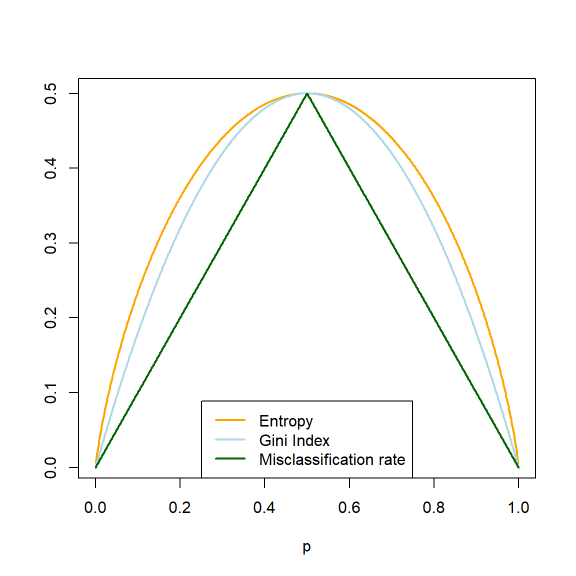
Figure 6.8: Gini index, (scaled) entropy, and classification error as a function of node impurity for a binary response.
As seen in Figure 6.8, the Gini index and entropy are computationally similar. In fact, the tree package in R uses Gini as a possible splitting criterion, but not entropy.
There are several sources on the topic that use ambiguous and, at times, contradictory terminology to refer to Shannon entropy. For example, page 309 of Hastie et al. (2009) refers to the measurement in Equation (6.7) as “cross-entropy” or “deviance”, whilst Murphy (2013) uses the term “entropy”, but also equates it to deviance on page 547.
However, on page 221 of Hastie et al. (2009) we see that the term deviance is also used to refer to the quantity \(2 \times \text{NLL}\) (negative log-likelihood). In fact, it is the NLL that is known as cross-entropy (Bishop, 2006, p. 209). Cross-entropy11 is usually used as a measure of dissimilarity between two probability distributions, typically the predicted class probabilities and the true class probabilities, in which case this loss function is also referred to as “log loss”.
Deviance, which is proportional to NLL, therefore offers a likelihood-based approach to measuring node impurity.
3. Deviance
The deviance is constructed by viewing a classification tree as a probability model. Let \(\boldsymbol{Y}_m\), denoting the set of categorical responses in leaf node \(m\), be a random sample of size \(n_m\) from the multinomial distribution:
\[\begin{equation} p(\boldsymbol{y}_m) = \binom{n_m}{n_{m1} \cdots n_{mK} } \prod_{k=1}^{K} p_{mk}^{n_{mk}}. \tag{6.8} \end{equation}\]The likelihood over all \(M\) leaf nodes is then given by
\[\begin{equation} L = \prod_{m=1}^{M} p(\boldsymbol{y}_m) \propto \prod_{m=1}^{M} \prod_{k=1}^{K} p_{mk}^{n_{mk}}. \tag{6.9} \end{equation}\]Now, the deviance is defined as
\[\begin{equation} D = -2\log(L) = -2 \sum_{m=1}^{M} \sum_{k=1}^{K} n_{mk} \log(p_{mk}). \tag{6.10} \end{equation}\]We want the model that makes the data most probable, i.e. has the highest likelihood. This is equivalent to minimising the deviance. When we grow a classification tree, we therefore choose the split that reduces the deviance by the most at each step. Note that the deviance takes the number of observations in each terminal node into account, unlike the Gini index and entropy.
6.2.2 Link between deviance and RSS
Returning to regression trees for a moment, if we inspect the object created by the tree() function for the California housing data, we note that the RSS is actually referred to as “deviance” in the model output.
##
## Regression tree:
## tree(formula = HousePrice ~ Latitude + Longitude, data = calif)
## Number of terminal nodes:  12
## Residual mean deviance:  0.1662 = 3429 / 20630
## Distribution of residuals:
##     Min.  1st Qu.   Median     Mean  3rd Qu.     Max.
## -2.75900 -0.26080 -0.01359 0.00000 0.26310 1.84100## [1] 3428.558To make the link between the deviance of a classification tree and the RSS of a regression tree, suppose that for terminal node \(m\) the continuous response \(\boldsymbol{Y}_m\) is a random sample of size \(n_m\) from \(N(\mu_m, \sigma^2)\), such that the joint distribution of \(\boldsymbol{Y}_m\) is
\[\begin{equation} f(\boldsymbol{y}_m) = \left(\frac{1}{\sigma \sqrt{2\pi}} \right)^{n_m} \exp \left(\frac{-\sum_{i:x_i\in R_m} (y_i - \mu_m)^2}{2\sigma^2} \right). \tag{6.11} \end{equation}\]Since we are effectively modelling the \(\mu_m\), the likelihood of the means over all \(M\) leaf nodes is given by
\[\begin{equation} L(\boldsymbol{\mu}|\boldsymbol{x}) = \prod_{m=1}^{M} f(\boldsymbol{y}_m) \propto \exp \left(-\frac{1}{2}\sum_{m=1}^{M}\sum_{i:x_i\in R_m} (y_i - \mu_m)^2 \right), \tag{6.12} \end{equation}\]such that the deviance can be expressed as
\[\begin{equation} D = -2\log(L) \propto \sum_{m=1}^{M}\sum_{i:x_i\in R_m} (y_i - \mu_m)^2 = RSS. \tag{6.13} \end{equation}\]Since the deviance is directly proportional to the RSS in this setting, minimising the one is equivalent to minimising the other.
Let us turn our attention back to classification trees and consider managing their complexity.
6.2.3 Cost complexity pruning
Just like with regression trees, we must prune a fully grown classification tree to avoid overfitting. However, as with the splitting rules, we cannot use the \(RSS_{\alpha}\) criterion for pruning when the response is categorical. Similar to regression trees though, we will again minimise a specified cost complexity criterion, penalised according to the size of the tree, \(|T|\):
\[\begin{equation} C_{\alpha}(T) = C(T) + \alpha|T|, \tag{6.14} \end{equation}\]where \(C(T)\) represents a chosen cost function. Although we could use any of the aforementioned criteria, if prediction accuracy of the final pruned tree is the goal, then \(C(T)\) should be taken as the misclassification rate of tree \(T\).
The following section illustrates the application to a binary classification problem.
6.2.4 Example 7 – Titanic
The famous Titanic dataset contains information on 891 passengers that were aboard the Titanic on its one and only trans-Atlantic journey. The goal is to predict survival (yes/no) based on the predictors shown in the following table:
titanic <- read.csv('data/titanic.csv', stringsAsFactors = T)
titanic$Pclass <- as.factor(titanic$Pclass) #Class coded as integer, should be factor
datatable(titanic, options = list(scrollX = T, pageLength = 6))
Most of the features are self-explanatory. SibSp refers to the passenger’s number of siblings plus spouses on board; Parch to their number of parents and children; and Embarked to their port of embarkation12.
To start with, we will first fit a classification tree using Gini index as splitting criterion.
titanic_tree_gini <- tree(Survived ~ ., data = titanic, split = 'gini')
plot(titanic_tree_gini)
text(titanic_tree_gini, pretty = 0)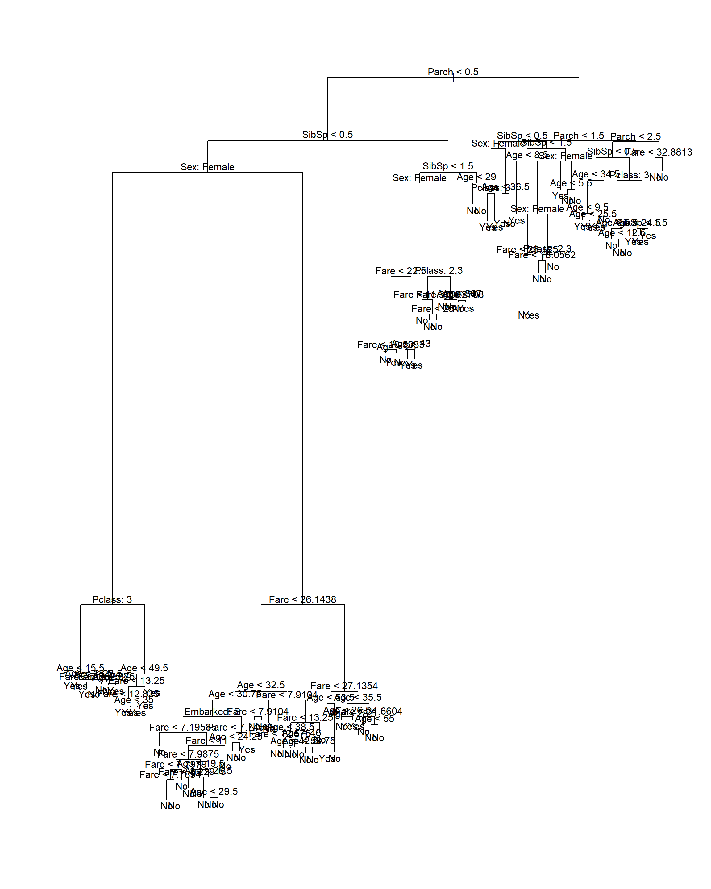
Figure 6.9: Classification tree fitted to the Titanic dataset using Gini index as splitting criterion
This yields a rather large tree, where the most useful feature (sex) is only used after a few prior splits. Compare this to the tree resulting from using deviance as splitting criterion (the default in the tree package), shown in Figure 6.10.
titanic_tree <- tree(Survived ~ ., data = titanic)
plot(titanic_tree)
text(titanic_tree, pretty = 0)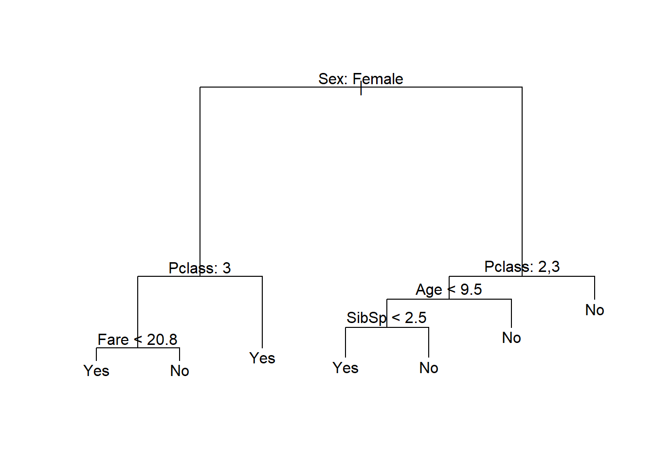
Figure 6.10: Classification tree fitted to the Titanic dataset using deviance as splitting criterion
This presents a similar picture to what one would expect given the emergency protocol of “women and children first”, although age was only an important factor for 2nd and 3rd class male passengers. We can extract any information for any of the nodes from the fitted object, or add different labels to the terminal nodes (see ?text.tree).
As a brief detour, let us show that the deviance measurement provided by the model’s summary indeed matches the definition set out in Equation (6.10). We will use the frame object contained in the model object to calculate the total deviance of the tree shown in Figure 6.10.
f <- titanic_tree$frame                      #We need the n's and the probs
n_m <- f$n[f$var == '<leaf>']                #This is total n per leaf, not per class!
p_n <- f$yprob[,1][f$var == '<leaf>']        #Pr(no) for all leaf nodes
p_y <- f$yprob[,2][f$var == '<leaf>']        #Pr(yes) for all leaf nodes
nlp <- (n_m*p_n)*log(p_n)+(n_m*p_y)*log(p_y) #\sum_k (n_k log(p_k)) for all leaves
nlp[is.nan(nlp)] <- 0                        #Need to deal with log(0)
(D <- -2*sum(nlp))                           #Deviance
## [1] 563.8652Comparing this to the total deviance reported, we see that it indeed matches:
## [1] 563.8652Note that although the deviance splitting criterion is used in software implementation as was shown here, none of the aforementioned sources explicitly define this criterion in the relevant sections on classification trees.
Another way of exploring the fitted tree – more as an exploration tool as opposed to one for reporting – is to simply print the object:
## node), split, n, deviance, yval, (yprob)
##       * denotes terminal node
##
##  1) root 714 964.500 No ( 0.59384 0.40616 )
##    2) Sex: Female 261 290.800 Yes ( 0.24521 0.75479 )
##      4) Pclass: 3 102 140.800 No ( 0.53922 0.46078 )
##        8) Fare < 20.8 79 108.500 Yes ( 0.44304 0.55696 ) *
##        9) Fare > 20.8 23  17.810 No ( 0.86957 0.13043 ) *
##      5) Pclass: 1,2 159  69.170 Yes ( 0.05660 0.94340 ) *
##    3) Sex: Male 453 459.900 No ( 0.79470 0.20530 )
##      6) Pclass: 2,3 352 298.300 No ( 0.84943 0.15057 )
##       12) Age < 9.5 30  41.050 Yes ( 0.43333 0.56667 )
##         24) SibSp < 2.5 16   0.000 Yes ( 0.00000 1.00000 ) *
##         25) SibSp > 2.5 14   7.205 No ( 0.92857 0.07143 ) *
##       13) Age > 9.5 322 225.600 No ( 0.88820 0.11180 ) *
##      7) Pclass: 1 101 135.600 No ( 0.60396 0.39604 ) *
Here we can see the path containing male passengers of class 2 or 3, age \(\leq\) 9, and siblings \(\leq\) 2 had a total of 16 passengers…all of whom survived! The best way to gauge whether this is indeed a pattern in the data (as opposed to a seemingly significant pocket of random variation), is to use cross-validation to estimate out-of-sample performance for pruned trees of different sizes.
In the code below we see that one must specify the pruning cost complexity function, which we will set to the misclassification rate.
# First, grow a slightly larger tree
titanic_bigtree <- tree(Survived ~ ., data = titanic,
                        control = tree.control(nobs = nrow(na.omit(titanic)),
                                               mindev = 0.005))

# Then prune it down
set.seed(28)
titanic_cv <- cv.tree(titanic_bigtree, FUN = prune.misclass) #Use classification error rate for pruning

# Make the CV plot
plot(titanic_cv$size, titanic_cv$dev, type = 'o',
     pch = 16, col = 'navy', lwd = 2,
     xlab = 'Number of terminal nodes', ylab='CV error')

titanic_cv$k[1] <- 0 #Don't want no -Inf
alpha <- round(titanic_cv$k,1)
axis(3, at = titanic_cv$size, lab = alpha, cex.axis = 0.8)
mtext(expression(alpha), 3, line = 2.5, cex = 1.2)
axis(side = 1, at = 1:max(titanic_cv$size))

T <- titanic_cv$size[which.min(titanic_cv$dev)] #The minimum CV Error
abline(v = T, lty = 2, lwd = 2, col = 'red')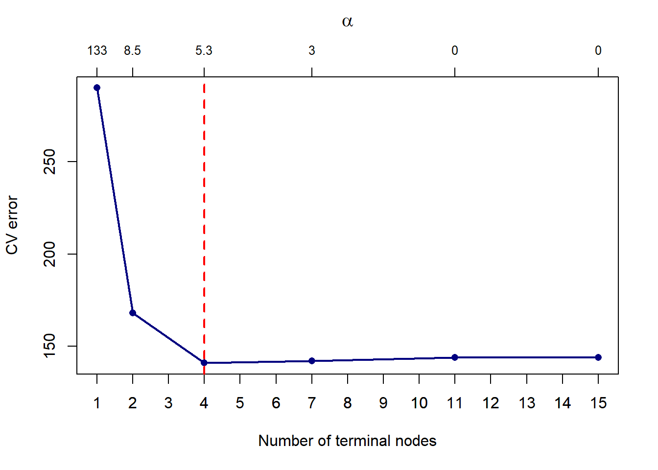
Figure 6.11: Cross-validated pruning results on a classification tree fitted to the Titanic dataset
For the specific seed set above, we see that a more parsimonious model with 4 leaves yields a lower CV error, which in Figure 6.11 is given as the number of misclassifications on the y-axis. Note that different seeds will yield different result. Next we prune the tree down to 4 leaves and plot the result.
titanic_pruned <- prune.misclass(titanic_bigtree, best = T)
plot(titanic_pruned)
text(titanic_pruned, pretty = 0)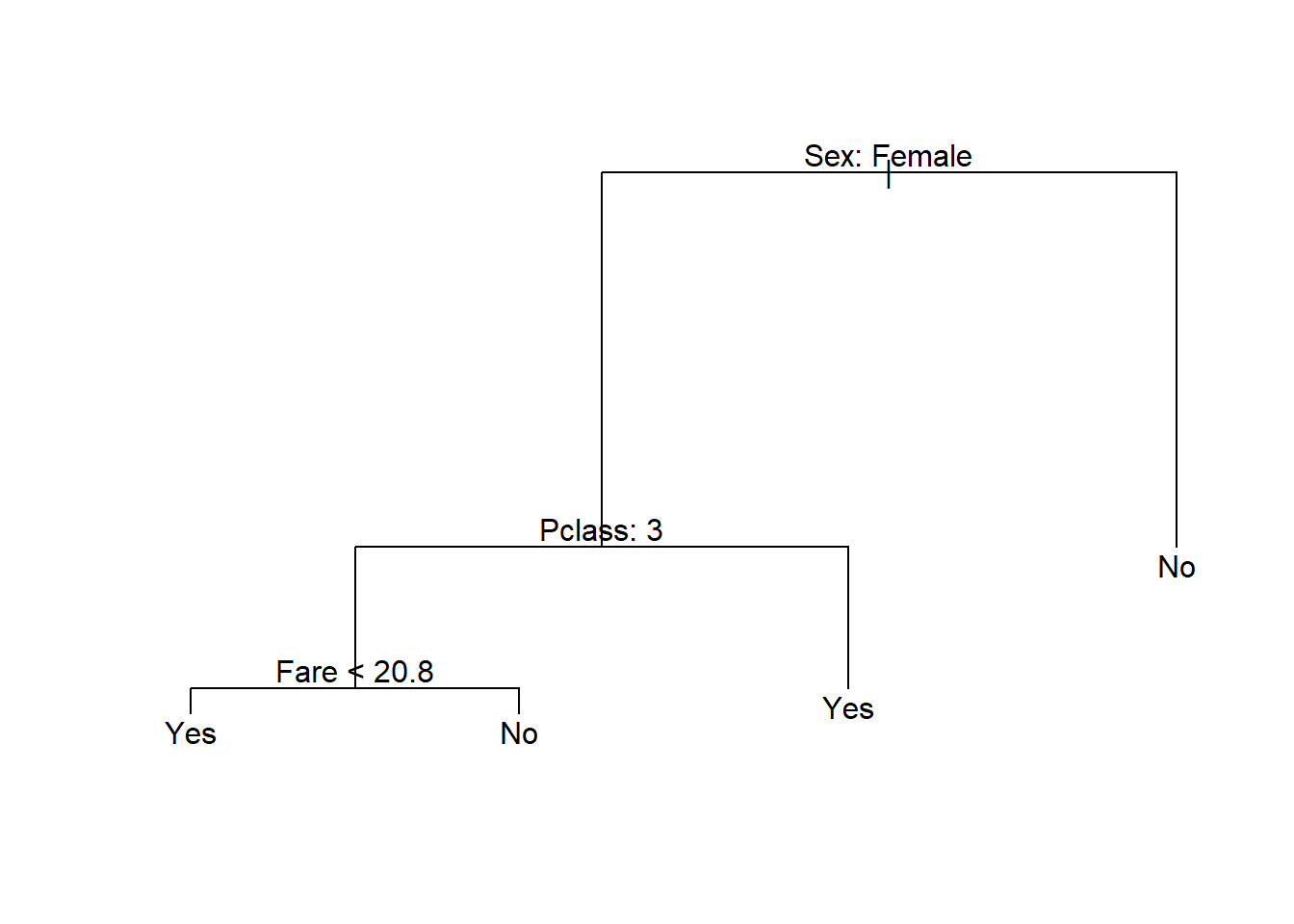
Figure 6.12: Pruned classification tree fitted to the Titanic dataset
From the resulting tree, all males would be classified as not surviving, together with female passengers in class 3 who’s fare was more than 20.8. We will once again not focus on prediction for single trees now, although we will include this as a benchmark when considering random forests and boosted trees.
In this example we saw that classification trees handle categorical predictors with ease, without the need to code dummy variables. Another benefit of this approach is that we can just as easily model target variables with multiple classes, as illustrated in the following example.
6.2.5 Example 8 – Iris
Another famous dataset, Iris contains data on 50 flowers from each of 3 species of iris. The measurements are on 4 features: sepal width, sepal length, petal width, and petal length. For the sake of illustrating the decision boundaries in two dimensions, we will only consider the sepal width and length. First, let’s plot the data:
# Load data
data('iris')

# Create index of species
ind <- as.numeric(iris$Species)

# Plot
plot(Sepal.Width ~ Sepal.Length, iris, xlab = 'Sepal Length', ylab = 'Sepal Width',
     col = c('red', 'green', 'blue')[ind],
     pch = c(1, 0, 5)[ind], lwd = 2, cex = 1.2)

legend(x = 'topright', legend = levels(iris$Species),
       pch = c(1, 0, 5), col = c('red', 'green', 'blue'), cex = 1.2)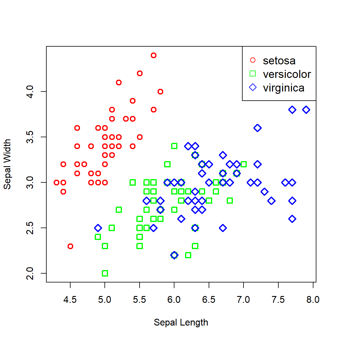
Figure 6.13: Iris data plotted across sepal width and length.
Now let’s fit a vanilla classification tree to the data and view the resulting partitioned feature space.
# Vanilla tree
iris_tree <- tree(Species ~ Sepal.Width + Sepal.Length, iris)

# Grid for predicting
x <- seq(min(iris$Sepal.Length), max(iris$Sepal.Length), length.out = 65)
y <- seq(min(iris$Sepal.Width), max(iris$Sepal.Width), length.out = 65)
fgrid <- expand.grid(Sepal.Length = x, Sepal.Width = y)

# Predict over entire space
iris_pred <- predict(iris_tree, fgrid, type = 'class')
ind_pred <- as.numeric(iris_pred)

# Custom colours
r <- rgb(255, 0, 0, maxColorValue = 255, alpha = 255*0.25)
g <- rgb(0, 255, 0, maxColorValue = 255, alpha = 255*0.25)
b <- rgb(0, 0, 255, maxColorValue = 255, alpha = 255*0.25)

# Plot the predicted classes
plot(fgrid$Sepal.Width ~ fgrid$Sepal.Length,
     col = c(r, g, b)[ind_pred],
     pch = 15, xlab = 'Sepal Length', ylab = 'Sepal Width')

# And add the data
points(Sepal.Width ~ Sepal.Length, iris,
       col = c('red', 'green', 'blue')[ind],
       pch = c(1, 0, 5)[ind], lwd = 2, cex = 1.2)

legend(x = 'topright', legend = levels(iris$Species),
       pch = c(1, 0, 5), col = c('red', 'green', 'blue'), cex = 1.2)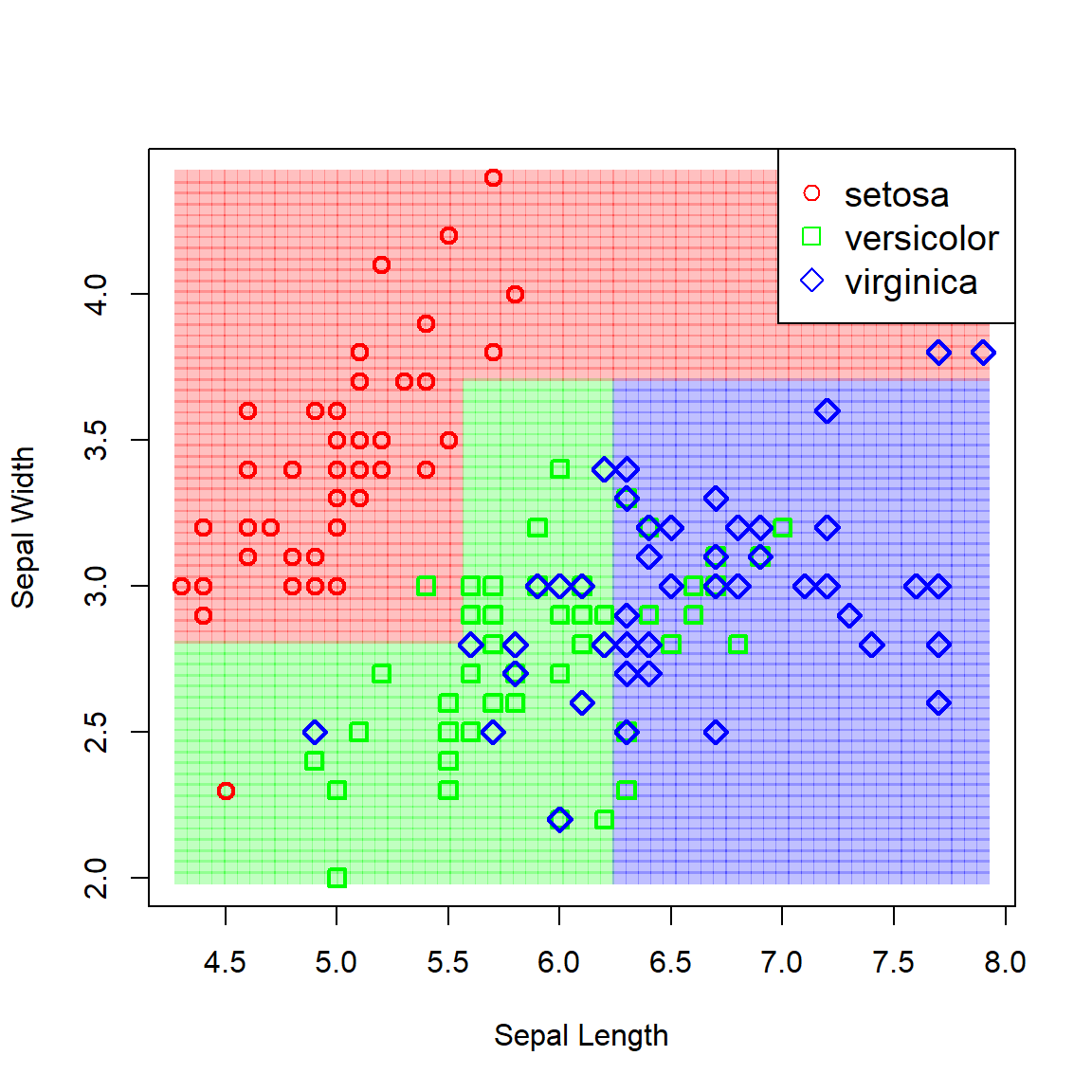
Figure 6.14: Partitioned feature space resulting from a vanilla classification tree fitted to the iris data.
Although these boundaries capture the underlying pattern seemingly well, we might well ask whether non-orthogonal boundaries would not have been more appropriate – either linear or non-linear. This raises the question of which approach/model is “best”.
The answer is that it depends on the problem. For some cases, a particular method might work well, whilst it is entirely inappropriate for others. Figure 6.15, taken from James et al. (2013), shows two hypothetical binary classification scenarios – one where a logistic regression will yield perfect separation whilst the classification tree struggles (top), and one where a classification tree requires only two splits to perfectly capture the decision boundaries, whilst logistic regression performs poorly.
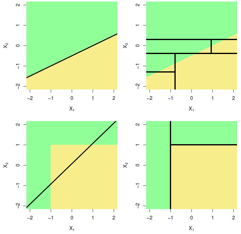
Figure 6.15: Top row: A hypothetical binary classification scenario in which logistic regression would outperform a decision tree. Bottom row: A different scenario in which the decision tree would outperform logistic regression. Source: James et al. (2013), p. 339.
Decision trees have some definite advantages:
They are very easy to explain and interpret – easier than linear regression!
Residual assumptions and multicollinearity are moot.
It mirrors human decision making.
Easily handle qualitative predictors without the need to create dummy variables.
However, one major drawback is that their predictive accuracy is generally (for most problems) not as good as most other regression and classification approaches. We will now consider two ways of improving on their predictive accuracy, namely random forests and boosting.
6.3 Bagging and random forests
The primary reason for the weak performance of decision trees on out-of-sample data is that they suffer from high sampling variability, especially on higher dimensional data. In other words, if we were to take different samples from the same population and fit trees to each sample, the results could look quite different, as seen in the following example.
For illustration purposes, consider the Sonar dataset contained in the mlbench package. The task is to determine whether sets of 60 sonar signals pertain to a metal cylinder/mine (M) or a roughly cylindrical rock (R). For every random 70/30 data split we fit a vanilla regression tree and track both the fitted tree and the resulting test classification accuracy.
library(mlbench)
library(maptree) #Better tree plotting
data(Sonar)
accs <- c()

par(mfrow=c(1,2))
set.seed(4026)

for (i in 1:100){
  # Split and fit
  train <- sample(1:nrow(Sonar), 0.7*nrow(Sonar))
  my_tree <- tree(formula = Class ~ ., data = Sonar, subset = train)

  # Predict and evaluate
  yhat <- predict(my_tree, Sonar[-train,], type = 'class')
  y <- Sonar[-train, 'Class']
  accs <- c(accs, sum(diag(table(y, yhat)))/length(y)*100)

  # Plots
  draw.tree(my_tree, cex = 0.5)
  plot(1:i, accs, type = 'o', pch = 16, xlab = '', ylab = 'Classification accuracy (%)',
       xlim = c(1, 100), ylim = c(50, 100))
}
Figure 6.16: Different trees and test accuracies resulting from different train/test splits on the Sonar dataset
Figure 6.16 shows how the fitted model and its testing accuracy can vary extensively across different random samples, with a classification accuracy range of 30.2% in these 100 samples. Although we can manage the complexity – and, therefore, the sampling variance – to some extent through pruning, bagging and random forests offer a much more effective approach.
6.3.1 Bagging
Before defining a random forest, we first need to explain the bagging procedure (we will shortly see that a bagged tree model is a special case of a random forest). Bootstrap aggregation, or bagging, is a general purpose procedure for reducing the variance of a statistical learning method by averaging over multiple predictions.
To illustrate the concept of variance reduction, consider a set of \(n\) independent observations \(X_1, \ldots, X_n\) each with variance \(\sigma^2\). It is well known that \(\text{var}\left({\bar{X}}\right) = \frac{\sigma^2}{n}\), i.e. averaging over multiple variables reduces the variance.
If we had \(B\) training sets, we could build a statistical model on each one and average the predictions on the test set:
\[\hat{y}_{\text{ave}} = \frac{1}{B} \sum_{b=1}^B \hat{y}_b\]
The average prediction \(\hat{y}_{\text{ave}}\) will therefore have a lower sampling variance than the prediction \(\hat{y}_b\) for any single training set.
However, we of course only have one sample in practice. This is where bootstrap sampling is useful: we can construct multiple bootstrap samples by repeated sampling with replacement from the training set, then grow \(B\) unpruned trees on each of these samples. For a continuous response variable we simply average the \(B\) predictions from the regression trees for each observation, whilst for categorical responses we take a majority vote, i.e. the overall prediction for an observation is the most commonly occurring category among the \(B\) predictions.
Figure 6.17 illustrates the process for a simple binary classification example with 5 observations and 3 trees. The default number of trees in most R packages is 500, which generally tends to be enough for the error to stabilise, depending on the size of the data. One can add more trees at extra computational cost, although note that since we are only reducing the prediction variability, a large value of \(B\) will not lead to overfitting.
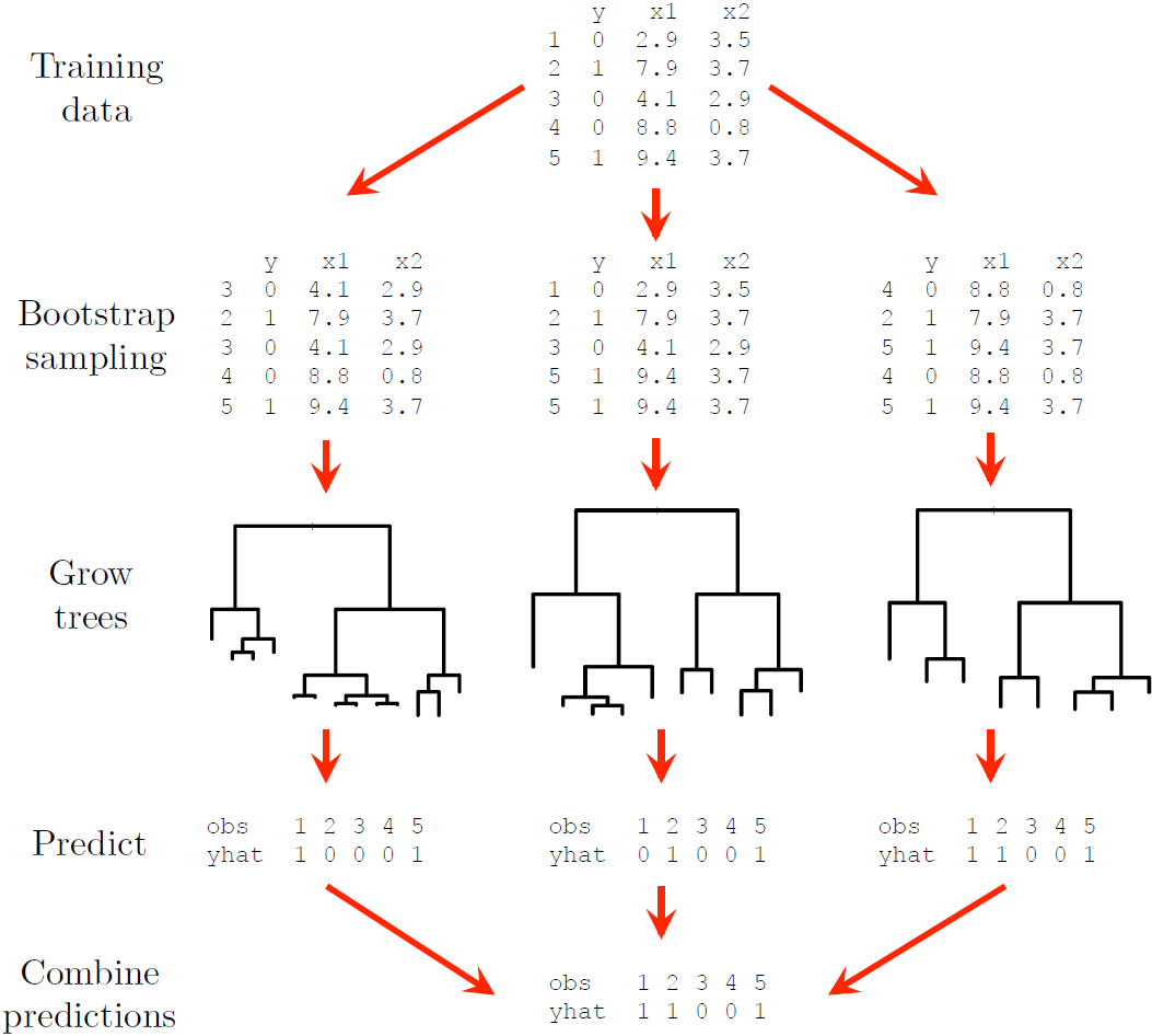
Figure 6.17: A dummy example illustrating the bagging procedure.
The benefit of the bagging procedure above a single tree is easily measured by out-of-sample performance, which in essence means that this procedure does better at capturing the true underlying relationship, \(f\). This is seen by investigating the decision boundaries, as shown for simulated linearly separable data in Figure 6.18.
library(randomForest)
par(mfrow = c(1, 2))

# Simulate random points
set.seed(123)
x1 <- runif(500, 0, 10)
x2 <- runif(500, 0, 10)
y <- as.factor(ifelse(x2 <= 10 - x1, 0, 1)) # With a linear decision boundary

# Tree first
mytree <- tree(y ~ x1 + x2, split = 'gini')

# Checked separately that 10 nodes is a good size (verify with cv.tree)
pruned_tree <- prune.tree(mytree, best = 10, method = 'misclass')
plot(x1, x2, col = ifelse(y == 0, 'red', 'navy'), pch = 16, xlim = c(0, 10), ylim = c(0, 10),
     xlab = expression(X[1]), ylab = '', cex.axis = 1.2, cex.lab = 1.5, asp = 1)
title(ylab = expression(X[2]), line = 1.8, cex.lab = 1.5) #ylab was being cut off

# Boundaries
abline(10, -1, lwd=3)
partition.tree(pruned_tree, add = T, lwd = 6, col = 'darkgreen', cex = 2)
x <- seq(0, 10, length = 100)
fgrid <- expand.grid(x1 = x, x2 = x)
yhat <- predict(pruned_tree, fgrid)[, 2]
contour(x, x, matrix(yhat, 100, 100), add = T,
        levels = 0.5, drawlabels = F, lwd = 4, col = 'darkgreen')

# Now bagged model (special case of random forest with m = p)
mybag <- randomForest(y ~ x1 + x2, mtry = 2)

# Plot
plot(x1, x2, col = ifelse(y == 0, 'red', 'navy'), pch = 16, xlim = c(0, 10), ylim = c(0, 10),
     xlab = expression(X[1]), ylab = '', cex.axis = 1.2, cex.lab = 1.5, asp = 1)
title(ylab = expression(X[2]), line = 1.8, cex.lab = 1.5) #ylab was being cut off

# Boundaries
abline(10, -1, lwd=3)
yhat <- predict(mybag, fgrid, type = 'prob')[, 2]
contour(x, x, matrix(yhat, 100, 100), add = T,
        levels = 0.5, drawlabels = F, lwd = 3, col = 'darkgreen')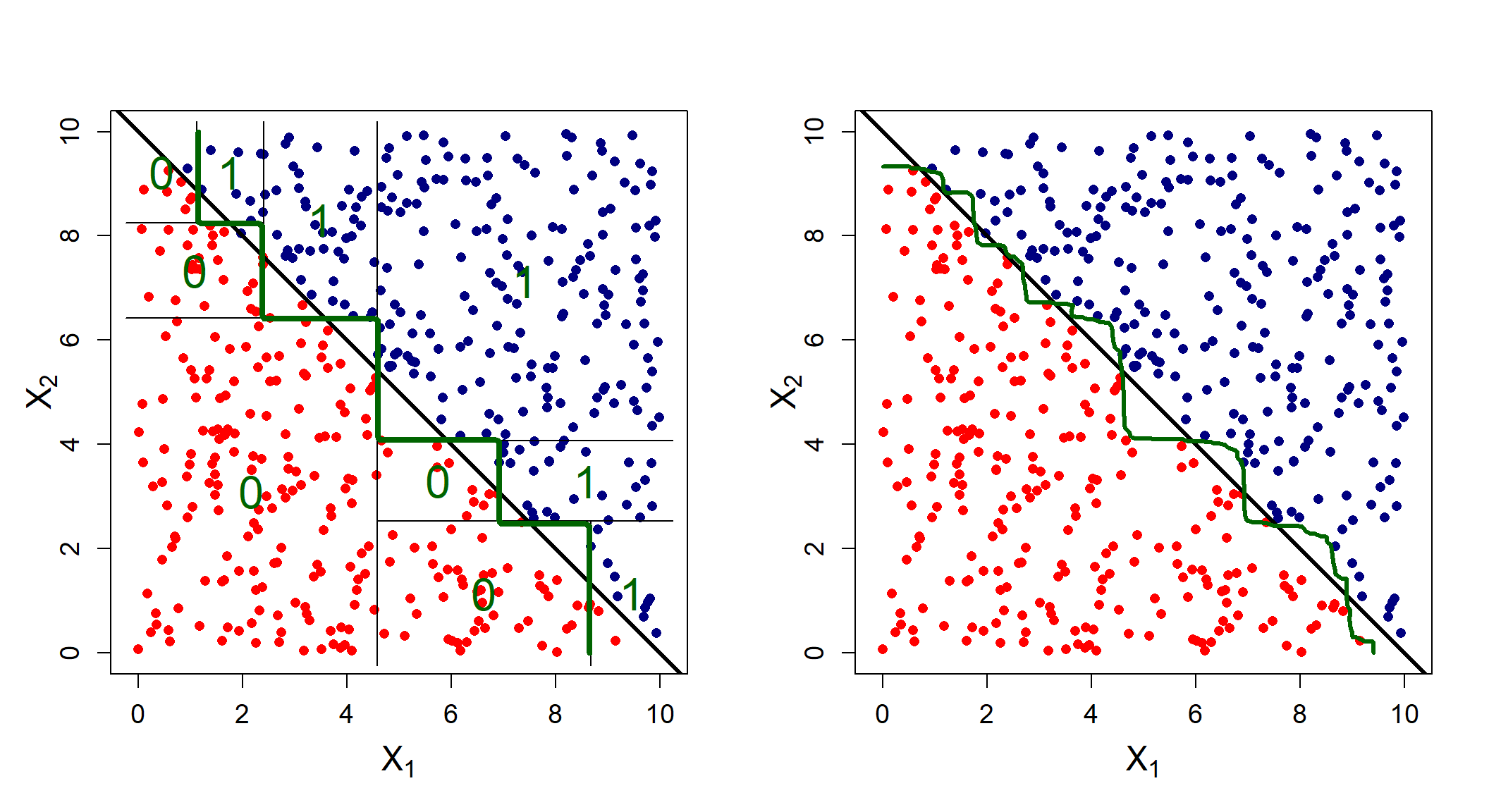
Figure 6.18: Estimated (green) vs actual (black) decision boundaries for a single tree (left) compared to a vanilla bagged model (right).
Here we see that the bagged model better approximates the decision boundary. Of course, one would rather fit a linear logistic regression to such a problem, but what about scenarios where the decision boundary is especially non-linear?
library(randomForest)
library(plotrix) #For drawing the circle
par(mfrow = c(1, 2))

# Simulate random points
set.seed(123)
x1 <- runif(1000, 0, 10)
x2 <- runif(1000, 0, 10)
circ <- (x1 - 5)^2 + (x2 - 5)^2
y <- as.factor(ifelse(circ <= 3^2, 0, 1))

# Tree first
mytree <- tree(y ~ x1 + x2)

# Checked separately that 5 nodes is a good size (verify with cv.tree)
pruned_tree <- prune.tree(mytree, best = 5, method = 'misclass')
plot(x1, x2, col = ifelse(y == 0, 'red', 'navy'), pch = 16, xlim = c(0, 10), ylim = c(0, 10),
     xlab = expression(X[1]), ylab = '', cex.axis = 1.2, cex.lab = 1.5, asp = 1)
title(ylab = expression(X[2]), line = 1.8, cex.lab = 1.5) #ylab was being cut off

# Boundaries
draw.circle(5, 5, 3, nv = 100, border = 'black', col = NA, lwd = 4)
partition.tree(pruned_tree, add = T, lwd = 6, col = 'darkgreen', cex = 2)
x <- seq(0, 10, length = 150)
fgrid <- expand.grid(x1 = x, x2 = x)
yhat <- predict(pruned_tree, fgrid)[, 2]
contour(x, x, matrix(yhat, 150, 150), add = T,
        levels = 0.5, drawlabels = F, lwd = 4, col = 'darkgreen')

# Now bagged model (special case of random forest with m = p)
mybag <- randomForest(y ~ x1 + x2, mtry = 2)

# Plot
plot(x1, x2, col = ifelse(y == 0, 'red', 'navy'), pch = 16, xlim = c(0, 10), ylim = c(0, 10),
     xlab = expression(X[1]), ylab = '', cex.axis = 1.2, cex.lab = 1.5, asp = 1)
title(ylab = expression(X[2]), line = 1.8, cex.lab = 1.5) #ylab was being cut off

# Boundaries
draw.circle(5, 5, 3, nv = 100, border = 'black', col = NA, lwd = 4)
yhat <- predict(mybag, fgrid, type = 'prob')[, 2]
contour(x, x, matrix(yhat, 150, 150), add = T,
        levels = 0.5, drawlabels = F, lwd = 3, col = 'darkgreen')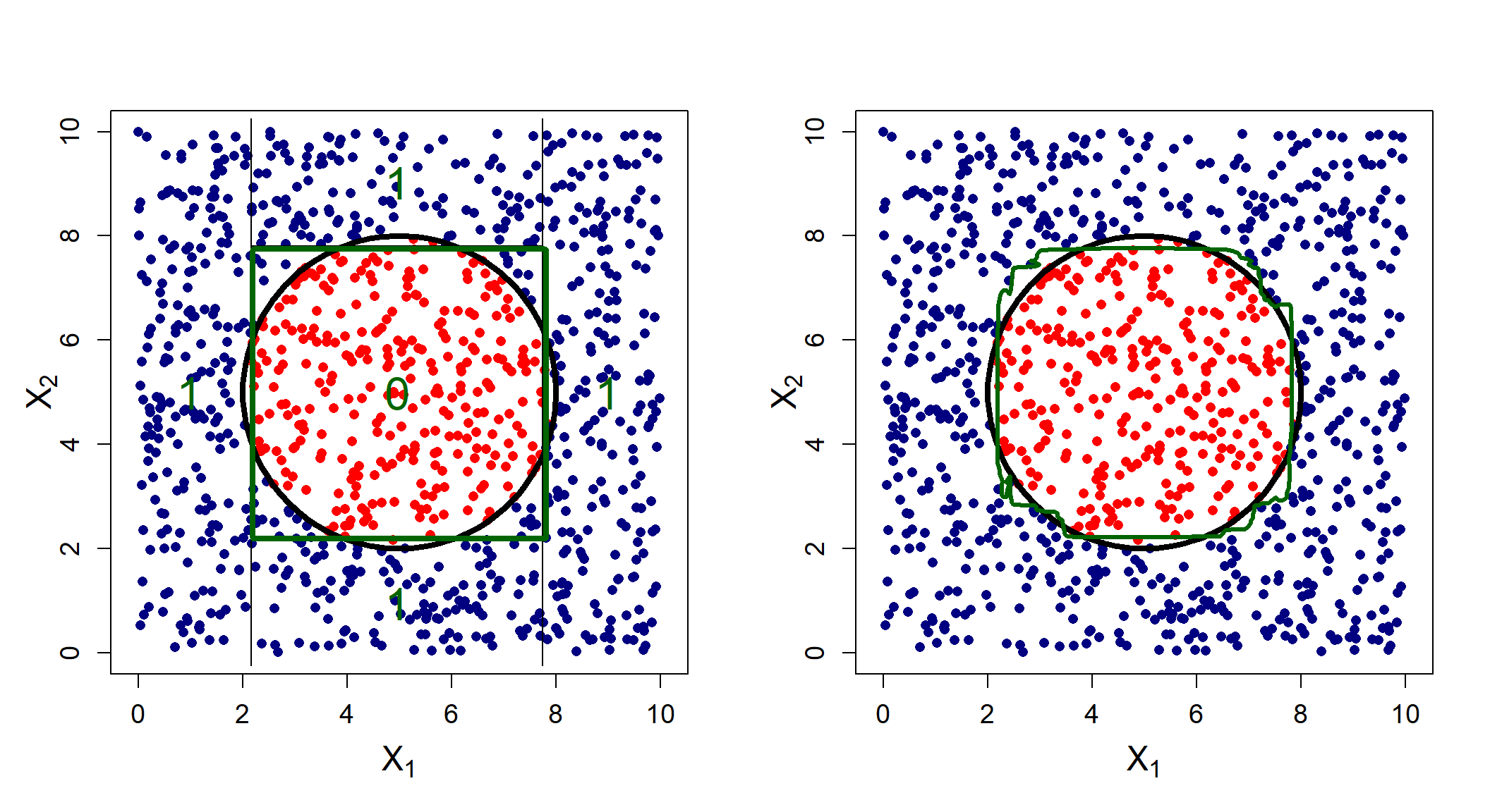
Figure 6.19: Estimated (green) vs actual (black) decision boundaries for a single tree (left) compared to a vanilla bagged model (right).
Figure 6.19 again shows that although the tree does roughly capture the overall pattern, its orthogonal splits struggle to capture the circular boundary, whereas the bagged model adjusts appropriately to some extent.
6.3.2 Out-of-bag error estimation
One convenient upshot of this approach is the built-in capability of estimating the test error without the need for cross-validation. This is due to the fact that each bagged tree only uses approximately 2/3 of the observations on average \(\left(\frac{e-1}{e}\text{, to be exact}\right)\). The remaining ~1/3 observations \(\left(\frac{1}{e}\right)\) not used to grow a bagged tree are called out-of-bag (OOB) observations.
To obtain an estimate of the test error, we simply predict the response for observation \(i\) using each of the bagged trees for which that observation was OOB. This will yield approximately \(\frac{B}{3}\) predictions per observation, which are then combined into a single prediction per observation by either computing the OOB RSS (regression trees) or OOB classification error (classification trees). Since this error rate is based on out-of-sample observations, it serves as an estimate of the test error, just like cross-validation errors.
Figure 6.20 again illustrates the process for a simple regression example (note that some rounding was applied for ease of presentation).
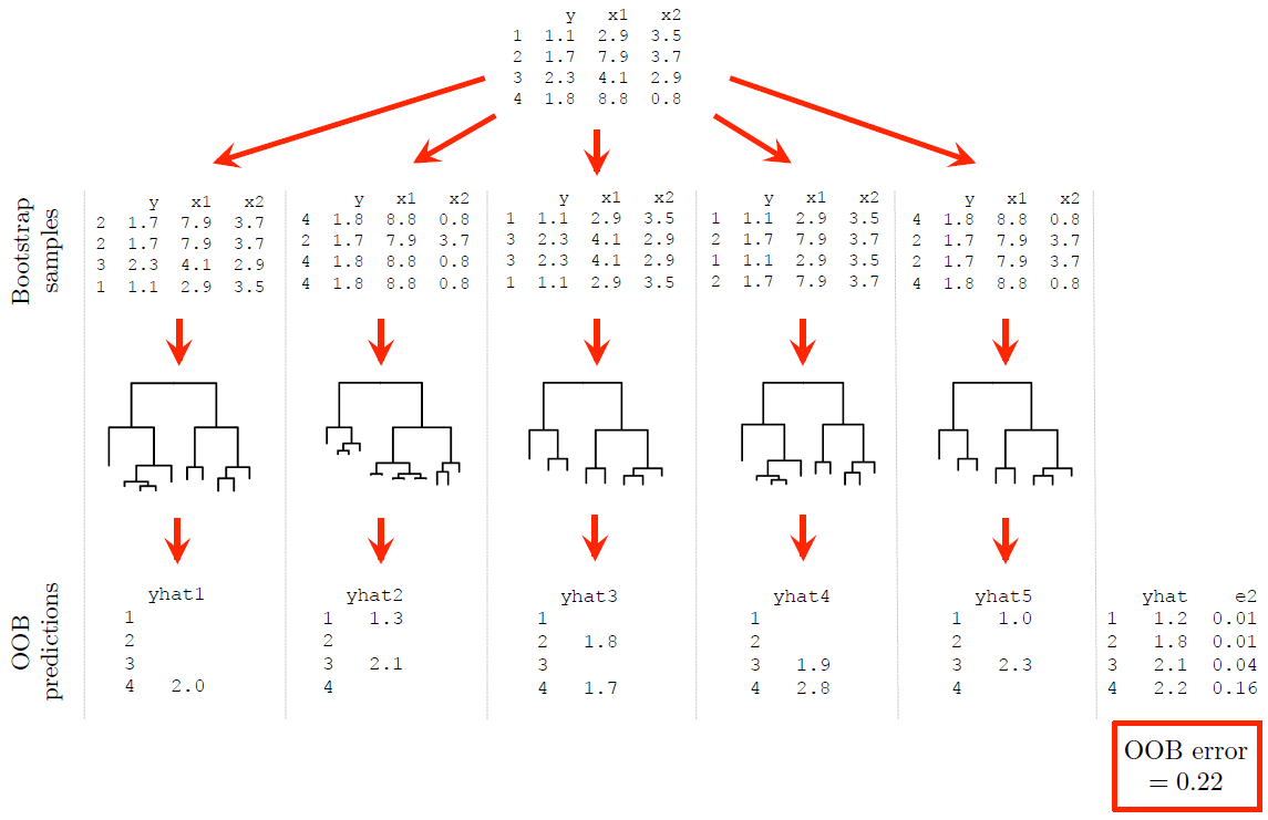
Figure 6.20: A dummy example illustrating out-of-bag (OOB) error estimation.
6.3.3 Variable importance
When we bag a large number of trees, we lose some of the interpretation qualities of decision trees since it is no longer possible to represent the model with a single tree. We can, however, measure the variable importance for each predictor.
The two most commonly reported measures are impurity-based importance and permutation importance. Although they often lead to similar rankings, they quantify importance in fundamentally different ways.
Impurity-based importance (Mean Decrease in Impurity)
Each split in a regression tree reduces the residual sum of squares (RSS). In a random forest, we can aggregate the total reduction in RSS attributable to a predictor across all trees and all splits. The importance of variable \(X_j\) is therefore
\[ \text{VI}_j = \sum_{\text{trees}} \sum_{\text{splits on } X_j} \Delta \text{RSS}. \]
This measures how much the variable contributes to reducing training error during tree construction. The advantage of this approach is that it is computationally inexpensive, since the reductions are already calculated when the trees are grown. However, it is known to be biased in favour of continuous variables or predictors with many possible split points, since these have more opportunities to achieve large impurity reductions.
Permutation importance (Mean Decrease in Accuracy)
Permutation importance measures the increase in prediction error when the values of a predictor are randomly permuted. After the model has been fitted, we:
- Compute the baseline prediction error.
- Randomly shuffle the values of \(X_j\) in the validation (or out-of-bag) data.
- Recompute the prediction error.
- Attribute the increase in error to the importance of \(X_j\).
Formally, if \(\text{Err}\) denotes the prediction error, then
\[ \text{VI}_j = \text{Err}_{\text{perm}(X_j)} - \text{Err}_{\text{original}}. \]
This measure is directly tied to predictive performance and quantifies how much model performance deteriorates when the information contained in \(X_j\) is removed. Its main drawback is that it is computationally more expensive and can be unstable in the presence of highly correlated predictors, since other variables may partially compensate for the permuted feature.
In practice, both measures aim to quantify the contribution of each predictor, but they reflect different aspects of the model: impurity-based importance reflects the internal mechanics of tree construction, whereas permutation importance reflects the impact of a variable on predictive performance.
Now that we have motivated for bagged trees and explored some of their uses, we will make one tweak to the algorithm, thereby defining random forests.
6.3.4 Random forests
We have established that bagging reduces the sampling variability of predictions by averaging over many trees. However, if the trees are highly correlated, this improvement will be limited.
Consider again a set of random variables \(X_1, \ldots, X_n\) with common variance \(\sigma^2\), but this time suppose they are not independent, such that there is some non-zero correlation. We have that
\[\text{var}\left({\bar{X}}\right) = \frac{\sigma^2}{n} + \frac{2\sigma^2}{n^2} \sum_{i\ne j} \rho_{ij}.\] Therefore, the stronger the correlation, the greater the variance of the average. Random forests provide an improvement over bagged trees by making a small change that decorrelates the trees.
Suppose that there is one very strong predictor in a dataset – most of the bagged trees will use this predictor. Consequently, the bagged trees will look quite similar to each other and their predictions will therefore be highly correlated. As with bagging, a random forest is constructed by growing \(B\) decision trees on \(B\) bootstrapped samples. However, each time a split is considered, a random sample of \(m < p\) predictors are chosen as split candidates such that, on average, \(\frac{p-m}{p}\) of the splits will not even consider the strong predictor.
This has the effect of decorrelating the trees, causing the average predictions to be less variable between samples, thereby further reducing the variance component of the total error. In the R package randomForest (amongst others) the default is \(m = \lfloor \sqrt{p} \rfloor\) for classification trees and \(m = \lfloor p/3 \rfloor\) for regression trees.
Note that bagging is a special case of a random forest with \(m = p\). As with bagging, we can estimate the testing error by means of the OOB errors and we can also report the importance of each predictor across all splits across all trees in the forest. We will explore the application by returning to the earlier examples for both regression and classification.
6.3.5 Example 6 – California housing (continued)
After applying an 80/20 data split into training and testing sets, we will start by using the randomForest package to fit both a vanilla random forest and a bagged model to the California housing dataset, both using 250 trees. We will also keep track of the training times13.
# Train/test split
set.seed(4026)
train <- sample(1:nrow(calif), 0.8*nrow(calif))

# Bagging
bag_250_time <- system.time(
  calif_bag <- randomForest(HousePrice ~ ., data = calif, subset = train,
                            mtry = ncol(calif) - 1, #Use all features (minus response)
                            ntree = 250,
                            importance = T,         #Keep track of importance (faster without)
                            #do.trace = 25,         #Can keep track of progress if we want
                            na.action = na.exclude)
)

# Random Forest
rf_250_time <- system.time(
  calif_rf <- randomForest(HousePrice ~ ., data = calif, subset = train,
                           ntree = 250,
                           importance = T,
                           na.action = na.exclude)
)
From the model object we can extract much information on the fit (see calif_rf$...). For example, we can see that the random forest’s trees contained on average 10985 terminal nodes! We can also look at the percentage of variation in \(Y\) captured by the model, i.e. the coefficient of determination (\(R^2\)), by just printing the model object:
##
## Call:
##  randomForest(formula = HousePrice ~ ., data = calif, mtry = ncol(calif) -      1, ntree = 250, importance = T, subset = train, na.action = na.exclude)
##                Type of random forest: regression
##                      Number of trees: 250
## No. of variables tried at each split: 8
##
##           Mean of squared residuals: 0.05236698
## % Var explained: 83.83##
## Call:
## randomForest(formula = HousePrice ~ ., data = calif, ntree = 250, importance = T, subset = train, na.action = na.exclude)
## Type of random forest: regression
## Number of trees: 250
## No. of variables tried at each split: 2
##
## Mean of squared residuals: 0.05985603
## % Var explained: 81.52Verifying this calculation manually (just for the random forest model):
y_calif <- calif[train, ]$HousePrice
yhat_calif_rf <- calif_rf$predicted
# Calculate SSR = 1 - SSE/SST
round((1 - sum((y_calif - yhat_calif_rf)^2)/sum((y_calif - mean(y_calif))^2))*100, 2)
## [1] 81.52Interestingly, we see that the bagged model has the higher \(R^2\). Comparing their OOB error plots, we see that the bagged model also yields better (lower) errors:
plot(calif_bag$mse, type = 'l', xlab = 'Number of trees', ylab = 'OOB MSE',
     col = 'blue', lwd = 2, ylim = c(0, max(calif_rf$mse)))
lines(calif_rf$mse, col = 'darkgreen', lwd = 2, type = 's')
legend('topright', legend = c('Bagging', 'Random Forest'),
       col = c('blue', 'darkgreen'), lwd = 2)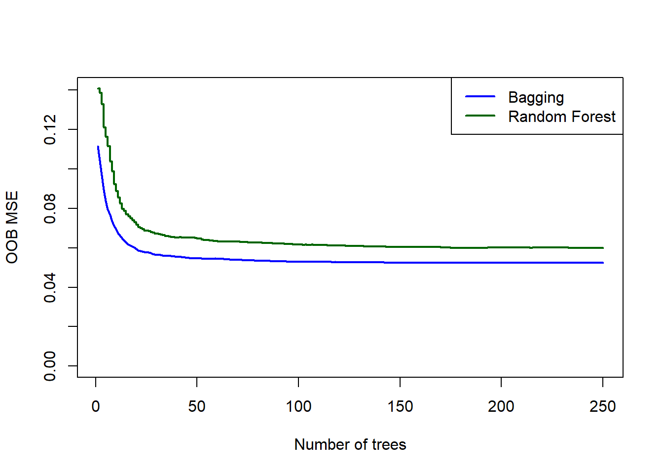
Figure 6.21: OOB errors for the bagged tree and random forest (default m) fitted to the California housing dataset.
Based on this, if we had to choose a model between these two, we would pick the bagged model. We will, however, apply both to the test set to compare the OOB estimates to the observed test errors. For comparison, let us add the test error for a single pruned tree as well.
# Quick single tree
stopcrit <- tree.control(nobs = length(train), mindev = 0.002)
calif_tree_overfit <- tree(HousePrice ~ ., data = calif[-train, ], control = stopcrit)
set.seed(4026)
calif_cv <- cv.tree(calif_tree_overfit)
T <- calif_cv$size[which.min(calif_cv$dev)]
calif_pruned <- prune.tree(calif_tree_overfit, best = T)

# Predictions
calif_bag_pred  <- predict(calif_bag, newdata = calif[-train, ])
calif_rf_pred   <- predict(calif_rf, newdata = calif[-train, ])
calif_tree_pred <- predict(calif_pruned, newdata = calif[-train, ])

# Prediction accuracy
y_calif_test   <- calif[-train, 1]
calif_bag_mse  <- mean((y_calif_test - calif_bag_pred)^2)
calif_rf_mse   <- mean((y_calif_test - calif_rf_pred)^2)
calif_tree_mse <- mean((y_calif_test - calif_tree_pred)^2)

# Plot MSEs
plot(calif_bag$mse, type = 'l', xlab = 'Number of trees', ylab = 'MSE',
     col = 'blue', lwd = 2, ylim = c(0, calif_tree_mse*2))
lines(calif_rf$mse, col = 'darkgreen', lwd = 2)
abline(h = calif_bag_mse, col = 'blue', lty = 2, lwd = 2)
abline(h = calif_rf_mse, col = 'darkgreen', lty = 2, lwd = 2)
abline(h = calif_tree_mse, col = 'grey', lty = 2, lwd = 2)
legend('topright', legend = c('Bagging OOB', 'Bagging test', 'Random forest OOB', 'Random forest test', 'Single tree test'),
       col = c('blue', 'blue', 'darkgreen', 'darkgreen', 'grey'), lwd = 2, lty = c('solid', 'dashed', 'solid', 'dashed', 'dashed'))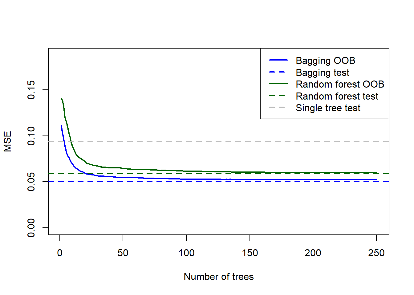
Figure 6.22: Testing errors for the bagged tree, random forest (default m), and single tree fitted to the California housing dataset, added to the OOB plots.
As expected, the model with \(m=8\) performed better on the test set. It is also interesting to note that for both models, the OOB error slightly overestimated the testing error. The bagged model’s test MSE of 0.05 is approximately half of the pruned regression tree test MSE (0.09).
Looking at the training times (in seconds), we see that it executed fairly quickly, even for this moderately-sized dataset:
##    user  system elapsed
## 111.49 0.27 111.99## user system elapsed
## 61.30 0.30 61.74The ranger package offers inter alia built-in parallelisation across cores to improve runtimes significantly. Fitting the bagged model using this package:
library(ranger)

ranger_time <- system.time(
  ranger_bag <- ranger(formula = HousePrice ~ .,
                       data = calif[train, ],
                       num.trees = 250,
                       mtry = ncol(calif) - 1)
)
We observe a significantly faster runtime:
##    user  system elapsed
##   19.77    0.53    1.69
The model object also has some neat output to explore. For example, let’s investigate the 100th tree in the forest:
##   nodeID leftChild rightChild splitvarID splitvarName splitval terminal prediction
## 1      0         1          2          0       Income  3.84240    FALSE         NA
## 2      1         3          4          0       Income  2.45985    FALSE         NA
## 3      2         5          6          0       Income  5.77605    FALSE         NA
## 4      3         7          8          6     Latitude 34.44500    FALSE         NA
## 5      4         9         10          6     Latitude 38.48500    FALSE         NA
## 6      5        11         12          1     HouseAge 38.50000    FALSE         NA
Note, however, that since the trees are fitted in parallel we cannot keep track of OOB MSE as the number of trees increase; we can only extract the final OOB MSE.
Another option for faster random forest implementation is Rborist. Wright & Ziegler (2017) compares the two packages across a range of combinations of observations and features. The result is neatly summarised in Figure 6.23, taken from that paper.
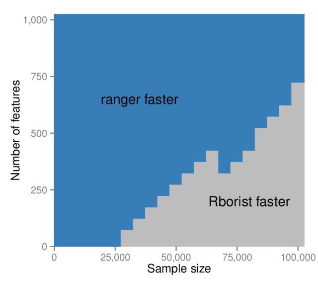
Figure 6.23: Runtime comparison of ranger with Rborist (classification, 1000 trees per run). Source: Wright & Ziegler (2017).
We see that for the California dataset, ranger will still be faster. We can now leverage the speed of this package to answer an important question, namely which value of \(m\) is best for this example. In the analyses above we only used \(m = p = 8\) and \(m = \lfloor p/3 \rfloor = 2\), but perhaps another value would yield better results. To determine this, we will use caret to perform a hyperparameter grid search (using ranger) across all possible values of \(m\). We can also control the tree depth, therefore we will try different size trees as well. We will again use 250 trees.
library(caret)
set.seed(1)

# Create combinations of hyperparameters
# see getModelInfo()$ranger$parameters
calif_rf_grid <- expand.grid(mtry = 2:(ncol(calif) - 1),
                             splitrule = 'variance',      #Must specify. This is RSS for regression
                             min.node.size = c(1, 5, 20)) #Default for regression is 5. Controls tree size

ctrl <- trainControl(method = 'oob', verboseIter = F)     #Can set to T to track progress

# Use ranger to run all these models
calif_rf_gridsearch <- train(HousePrice ~ .,
                             data = calif,
                             subset = train,
                             method = 'ranger',
                             num.trees = 250,
                             importance = 'impurity',
                             #verbose = T,
                             trControl = ctrl,
                             tuneGrid = calif_rf_grid)    #Here is the grid
The hyperparameter combination that yielded the best OOB result is as follows:
## Ranger result
##
## Call:
##  ranger::ranger(dependent.variable.name = ".outcome", data = x,      mtry = min(param$mtry, ncol(x)), min.node.size = param$min.node.size,      splitrule = as.character(param$splitrule), write.forest = TRUE,      probability = classProbs, ...)
##
## Type:                             Regression
## Number of trees:                  250
## Sample size:                      16512
## Number of independent variables:  8
## Mtry:                             7
## Target node size:                 5
## Variable importance mode:         impurity
## Splitrule:                        variance
## OOB prediction error (MSE):       0.05215617
## R squared (OOB):                  0.8389851
According to this process, the best random forest model was one with \(m =\) 7 and terminal nodes of size 5. A particularly useful feature of caret’s train() function is the trivially easy plotting of the hyperparameter tuning results, allowing one to see not only which combination was best, but also how it compared to others, as well as the effect of changing certain hyperparameters. This is shown in Figure 6.24.
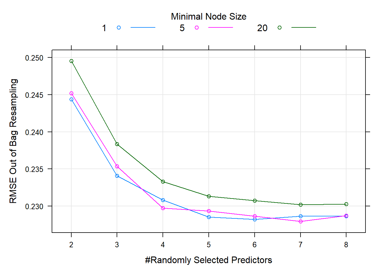
Figure 6.24: Hyperparameter combinations results for a random forest fitted to the California housing dataset.
There does not seem to be much difference between using entirely overfitted trees (minimal node size = 1) and ones with a minimal node size of 5, but increasing the node size to 20 (reducing the trees’ size) yielded worse performance for all values of \(m\). Although there is not much in it, we will now use the model that yielded the lowest OOB error to predict on the test set.
calif_rfgrid_pred <- predict(calif_rf_gridsearch, newdata = calif[-train,])
mean((y_calif_test - calif_rfgrid_pred)^2)
## [1] 0.05024634Comparing this to the \(m=8\) model from earlier, we see a miniscule improvement on its test MSE of 0.0502557, although the difference is negligible. To reiterate: in practice, one would only use the test set to get one final prediction after selecting a model based on CV/OOB errors. This test set comparison was merely for illustration.
Finally, let’s look at the variable importance plot. Although most packages contain their own built-in variable importance plotting functions, it is most convenient to use packages designed specifically for this purpose, like vip, to ensure standard presentation across different model classes. Note we measured impurity-based variable importance during training, which we can extract from the model object. We can use vi_permute() to calculate permutation importance (see an example of this later), or we can retrain the model and keep track of perumtation importance this time. Given the speed of ranger, we will do the latter here.
library(vip)
library(ggplot2)
library(patchwork) #Easy way to combine ggplots

calif_rf_besthp <- calif_rf_gridsearch$bestTune

calif_rf_perm <- ranger(
  HousePrice ~ .,
  data = calif[train, ],
  num.trees = 250,
  mtry = calif_rf_besthp$mtry,
  min.node.size = calif_rf_besthp$min.node.size,
  splitrule = calif_rf_besthp$splitrule,
  importance = 'permutation',
  seed = 123
)

crf_imp_p <- vip(calif_rf_gridsearch) +
  labs(
    title = 'Impurity Variable Importance',
    x = 'Increase in Prediction Error',
    y = NULL
  ) +
  theme_minimal()

crf_per_p <- vip(calif_rf_perm) +
  labs(
    title = 'Permutation Variable Importance',
    x = 'Decrease in Splitting Criterion',
    y = NULL
  ) +
  theme_minimal()

crf_per_p + crf_imp_p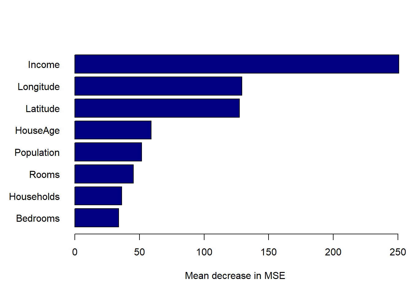
Figure 6.25: Variable importance plots for the tuned random forest fitted to the California housing dataset.
As expected, we see that median neighbourhood income yielded the greatest average reduction in RSS, during training followed by the location information. However, during permutation, removing only one of the location variables at a time did not have a major effect on prediction performance, presumably because much of the predictive power was still contained in the other location variable.
We can now apply the same procedure to the Titanic dataset.
6.3.6 Example 8 – Titanic (continued)
In practice one might want to jump straight to the hyperparameter tuning (after doing the necessary exploration and cleaning, of course). However, since we are still exploring and comparing these methods, we will again first see how the bagged model compares to the vanilla random forest, with a single pruned tree again added for reference. This step also helps to determine whether the number of trees is sufficient.
Since the Titanic dataset is much smaller than the California data, we will use a 70/30 split to be more certain of our out-of-sample performance.
# Train/test split
titanic <- na.omit(titanic)
set.seed(1)
train <- sample(1:nrow(titanic), 0.7*nrow(titanic))

# Bagging
titanic_bag <- randomForest(Survived ~ ., data = titanic, subset = train,
                            mtry = ncol(titanic) - 1,
                            ntree = 1000)

# Random Forest
titanic_rf <- randomForest(Survived ~ ., data = titanic, subset = train,
                           ntree = 1000)

# Quick single tree
stopcrit <- tree.control(nobs = length(train), mindev = 0.005)
titanic_tree_overfit <- tree(Survived ~ ., data = titanic, subset = train, control = stopcrit)
titanic_cv <- cv.tree(titanic_tree_overfit)
T <- titanic_cv$size[which.min(titanic_cv$dev)]
titanic_pruned <- prune.tree(titanic_tree_overfit, best = T)

# Predictions
titanic_bag_pred  <- predict(titanic_bag, newdata = titanic[-train, ])
titanic_rf_pred   <- predict(titanic_rf, newdata = titanic[-train, ])
titanic_tree_pred <- predict(titanic_pruned, newdata = titanic[-train, ], type = 'class')

# Prediction accuracy
y_titanic_test   <- titanic[-train, 1]
titanic_bag_mis  <- mean(y_titanic_test != titanic_bag_pred)
titanic_rf_mis   <- mean(y_titanic_test != titanic_rf_pred)
titanic_tree_mis <- mean(y_titanic_test != titanic_tree_pred)

# Plot errors
plot(titanic_rf$err.rate[, 'OOB'], xlab = 'Number of trees', ylab = 'Classification error',
     type = 's', col = 'darkgreen', ylim = c(0.1, titanic_tree_mis))
lines(titanic_bag$err.rate[, 'OOB'], col = 'blue', type = 's')
abline(h = titanic_bag_mis, col = 'blue', lty = 2, lwd = 2)
abline(h = titanic_rf_mis, col = 'darkgreen', lty = 2, lwd = 2)
abline(h = titanic_tree_mis, col = 'grey', lty = 2, lwd = 2)
legend('bottomright', legend = c('Bagging OOB', 'Bagging test', 'Random forest OOB', 'Random forest test', 'Single tree test'),
       col = c('blue', 'blue', 'darkgreen', 'darkgreen', 'grey'), lwd = 2, lty = c('solid', 'dashed', 'solid', 'dashed', 'dashed'))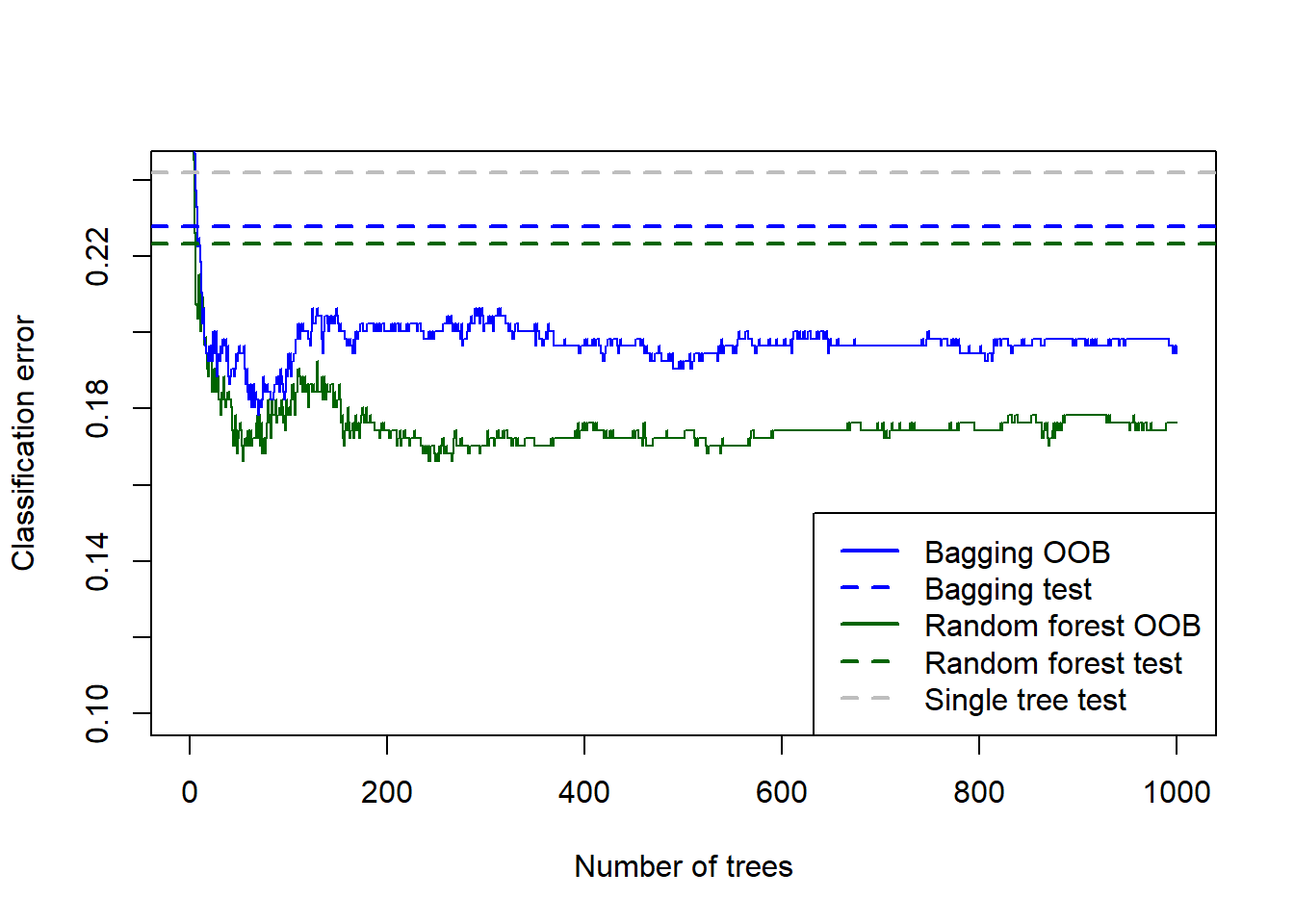
Figure 6.26: Testing errors for the bagged tree, random forest (default m), and single tree fitted to the Titanic dataset, added to the OOB error plots.
For this dataset – which is again considerably smaller than the California problem – we see that the OOB errors underestimated the testing errors. Although the default random forest was superior, we would again like to check all possible values of \(m\). We will also try two different splitting criteria: Gini index and Hellinger distance. See Aler et al. (2020) for information on the latter.
set.seed(2)

# Create combinations of hyperparameters
titanic_rf_grid <- expand.grid(mtry = 2:(ncol(titanic) - 1),
                               splitrule = c('gini', 'hellinger'),
                               min.node.size = c(1, 5, 10))

ctrl <- trainControl(method = 'oob', verboseIter = F)

# Use ranger to run all these models
titanic_rf_gridsearch <- train(Survived ~ .,
                               data = titanic,
                               subset = train,
                               method = 'ranger',
                               num.trees = 1000,
                               importance = 'permutation',
                               trControl = ctrl,
                               tuneGrid = titanic_rf_grid
)

plot(titanic_rf_gridsearch)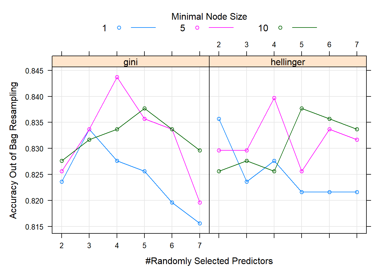
Figure 6.27: Hyperparameter combinations results for a random forest fitted to the Titanic dataset.
In Figure 6.27 we see that both splitting rules yield the highest accuracy when \(m=4\) and minimum node size is 5, with the Gini index split being superior at this combination. Note that these models fitted to a relatively small dataset like this one can be susceptible to sampling variation. As a homework exercise, rerun the above procedure multiple times and observe the change in results.
Next, we use the model that did best in OOB performance for prediction.
titanic_rfgrid_pred <- predict(titanic_rf_gridsearch, newdata = titanic[-train,])
titanic_rf_tuned_mis <- mean(y_titanic_test != titanic_rfgrid_pred)
Tuning the random forest’s hyperparameters brought the misclassification rate down from 22.33% to 21.4%.
Finally, let’s consider the variable importance plots. This time we only stored the permutation-based variable importance, hence we can retrain the best model and keep track of the impurity importance, should we want to view that as well.
titanic_rf_besthp <- titanic_rf_gridsearch$bestTune

titanic_rf_impurity <- ranger(
  Survived ~ .,
  data = titanic[train, ],
  num.trees = 1000,
  mtry = titanic_rf_besthp$mtry,
  min.node.size = titanic_rf_besthp$min.node.size,
  splitrule = titanic_rf_besthp$splitrule,
  importance = 'impurity',
  seed = 123
)

trf_per_p <- vip(titanic_rf_gridsearch) +
  labs(
    title = 'Permutation Variable Importance',
    x = 'Increase in Prediction Error',
    y = NULL
  ) +
  theme_minimal()

trf_imp_p <- vip(titanic_rf_impurity) +
  labs(
    title = 'Impurity Variable Importance',
    x = 'Decrease in Splitting Criterion',
    y = NULL
  ) +
  theme_minimal()

trf_per_p + trf_imp_p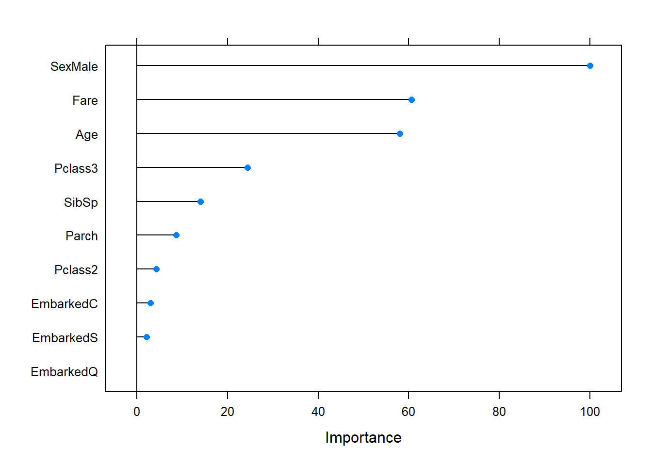
Figure 6.28: Variable importance plots for the tuned random forest fitted to the Titanic dataset.
Passenger sex is the most important factor according to both importance measures. Although passenger age yielded the second largest average decrease in Gini index during training, it is noticeably less important in prediction, where performance is measured according to classification accuracy. Fare also features prominently. Whether or not they were 3rd class passengers also had a notable impact on prediction accuracy (refer back to Figure 6.10, where we used the entire dataset).
Although there are many modern extensions to random forests, those will be left for future exploration. Our final topic in this section is another, different form of tree ensembling, namely boosting.
6.4 Gradient boosting
Boosting describes a general purpose family of algorithms that ensemble many weak learners into strong learners by letting the base models sequentially learn from the mistakes made by the previous ones, in contrast to bagging which grow all trees independently. The weak learner can be any classification or regression algorithm, but it is most common to use a decision tree, specifically one with few splits.
There are several boosting variations, the more popular ones being AdaBoost and so-called stochastic gradient boosting (it has been shown that this boosting can be interpreted as a form of gradient descent in function space). Our application will entail the latter, which is a more generic and flexible algorithm. Boosting can be applied to both regression and classification trees – which we will do – although our exploration of the algorithm will focus only on the regression case.
The main idea of boosting is to let the algorithm gradually learn from its mistakes by starting with a base prediction, for example the mean of the target variable. A regression tree with a small number of splits \((d)\), is fitted to the residuals of this base prediction. The (scaled) residuals of this tree are then treated as the response variable used to grow the next tree with \(d\) splits. The (scaled) residuals of the new tree are then used to grow another tree with \(d\) splits, and so on…
This yields a sequence of \(B\) trees, each one accounting for some of the variation in \(y\) that was not explained by the previous trees, gradually bringing the residuals down to zero. Therefore, the model eventually overfits as the number of trees increases, and we make use of cross-validation (CV) to determine at which point this occurs.
The initial trees will capture the strongest patterns in the data and will contribute the most to RSS reduction, whilst subsequent trees will lead to smaller improvements. We limit the rate of learning firstly by using trees with few splits, and secondly via a shrinkage parameter \(\lambda\) that down-weights the contribution of each tree. In general, methods that learn slowly tend to perform well, although this slow learning approach requires many more trees than a random forest.
The steps are laid out in the following algorithm:
Algorithm 1 Gradient Tree Boosting (as implemented in R)
Let \(\hat{y}^{(b)}\) be the predictions after fitting \(b\) trees
Let \(\hat{r}^{(b)}\) be the predicted values (of the residuals) of tree \(b\)
Let \(r^{(b)}\) be the residuals after fitting \(b\) trees
Set \(\hat{y}^{(0)} = \bar{y}\) such that \(r^{(0)} = y - \bar{y}\)
For \(b = 1, \ldots, B\):
- Fit a regression tree with \(d\) splits to \((X, r^{(b-1)})\)
- Using the predictions \(\hat{r}^{(b)}\) of the current tree, update the predictions \[\hat{y}^{(b)} = \hat{y}^{(b-1)} + \lambda\hat{r}^{(b)}\]
- Updated the residuals using the current predictions \[r^{(b)} = r^{(b-1)} - \lambda \hat{r}^{(b)}\]
- Calculate the model’s final predictions \[ \hat{y} = y - r^{(B)} = \bar{y} + \lambda \sum_{b=1}^{B} \hat{r}^{(b)} \]
This algorithm works remarkably well on a variety of problems despite (perhaps because of) its simplicity. In the code below we initiate the algorithm from scratch and apply it to a dummy data set.
library(rpart)
set.seed(4026)
n <- 100
x1 <- round(runif(n, 0, 10), 0)
x2 <- round(runif(n, 0, 10), 0)
y <- round(10 + 3*x1 + x2 + rnorm(n, 0, 10))
dat <- data.frame(cbind(y, x1, x2))

# Initiate algorithm "by hand"
gb.manual <- function(lambda, d, ntrees){
  train_mse <<- c()                     #To keep track of training error
  resids <<- c()                        #To keep track of residuals
  rhats <<- c()                         #To keep track of tree predictions

  yhat_b <- mean(y)                     #First initialisation of prediction -> step 1
  r_b <- y - yhat_b                     #First initialisation of residuals  -> step 1

  for(b in 1:ntrees){
    ctrl <- rpart.control(maxdepth = 1, cp = 0.001)
    t <- rpart(r_b ~ x1 + x2,
               control = ctrl)          #Fit tree to residuals              -> step 2a
    rhat_b <- predict(t, newdata = dat) #Predicted values of tree b         -> step 2b
    yhat_b <- yhat_b + lambda*rhat_b    #Updated prediction                 -> step 2b
    r_b <- y - yhat_b                   #Updated residuals                  -> step 2c
    # r_b <- r_b - lambda*rhat_b        #Could also write it like this, same thing

    # Save all the training mses, residuals, and tree predictions
    train_mse <<- c(train_mse, mean((y - yhat_b)^2)) #Double arrow saves object outside function
    resids <<- cbind(resids, r_b)
    rhats <<- cbind(rhats, rhat_b)
  }
  return(mean(y) + lambda*apply(rhats, 1, sum)) #Output final predictions   -> step 3
  # Could also return y - resids[, ntrees]
  # Or just yhat_b
}

#Run algorithm
yhat_manual <- gb.manual(lambda = 0.01, d = 1, ntrees = 1000)

#Final model training error
(gbm_manual_train_mse <- mean((y - yhat_manual)^2)) # Or just train_mse[ntrees]
## [1] 75.20785In order to validate this procedure, let us compare the results with those obtained from using the gbm package.
library(gbm) #No longer under development. Need to update to gbm3.
gbm_lib <- gbm(y ~ ., data = dat,
               distribution = 'gaussian', #Applies squared error loss
               n.trees = 1000,
               interaction.depth = 1,
               shrinkage = 0.01,
               bag.fraction = 1)          #Subsamples observations by default (0.5)

yhat_gbm <- gbm_lib$fit
(mse_gbm <- mean((y - yhat_gbm)^2))
## [1] 75.20785We see that the training MSEs match exactly. As a final sanity check, let’s compare each tree’s training error between the manual implementation and the package’s.
## [1] TRUEIn the above algorithm description and example we see that there are three main hyperparameters that must be specified beforehand:
- The number of trees – \(B\)
Unlike bagging and random forests, boosting can lead to overfitting if \(B\) is too large. We use cross-validation to select \(B\).
- The shrinkage parameter or learning rate – \(\lambda\)
Typical values are 0.01 or 0.001 (the default in gbm). Smaller values require more trees.
- The maximum number of splits in each tree – \(d\)
Also called the interaction depth of the boosted model, since \(d\) splits can involve at most \(d\) variables. Depending on the size of the problem, \(d=1\) can work well when fitting many trees.
Although these are the main hyperparameters, one can also further control the tree depth (useful when larger trees are preferred), as well as introduce randomisation by randomly subsampling the training set, somewhat reminiscent of the bagging process.
To illustrate the application, let us return to the California housing example.
6.4.1 Example 6 – California housing (continued)
Since this is our final analysis of this dataset, we will apply some feature engineering, a process of adapting/transforming/combining the existing information into new features to improve model performance.
Instead of using the total number of bedrooms, bathrooms, and people per neighbourhood, let’s use the number of households to convert these into per-house rates. We will also apply a 70/30 train/test split, here showing how a caret function can be used to do so.
library(dplyr)

# Create calif feature engineered
calif_fe <- calif %>% mutate(AveRooms = Rooms/Households,
                             AveBedrms = Bedrooms/Households,
                             AveOccup = Population/Households) %>%
  select(-Rooms, -Bedrooms, -Households)

# Using caret for train/test split:
set.seed(4026)
train_index <- createDataPartition(y = calif_fe$HousePrice, p = 0.8, list = FALSE)
calif_fe_train <- calif_fe[train_index,]
calif_fe_test <- calif_fe[-train_index,]
As some benchmark for comparison – and to see whether the engineered features are useful – we will first fit a single regression tree.
# Slightly larger tree
calif_fe_tree <- tree(HousePrice ~ ., data = calif_fe_train,
                      control = tree.control(nobs=nrow(calif),
                                             mindev = 0.003))

# Tune
set.seed(1)
calif_fe_cv <- cv.tree(calif_fe_tree)
calif_fe_cv$k[1] <- 0

plot(calif_fe_cv$size, calif_fe_cv$dev, type = 'o',
     pch = 16, col = 'navy', lwd = 2,
     xlab = 'Number of terminal nodes', ylab = 'CV RSS')
axis(side = 1, at = 1:max(calif_fe_cv$size), labels = 1:max(calif_fe_cv$size))
alpha <- round(calif_fe_cv$k)
axis(3, at = calif_fe_cv$size, lab = alpha)
mtext(expression(alpha), 3, line = 2.5, cex = 1.5)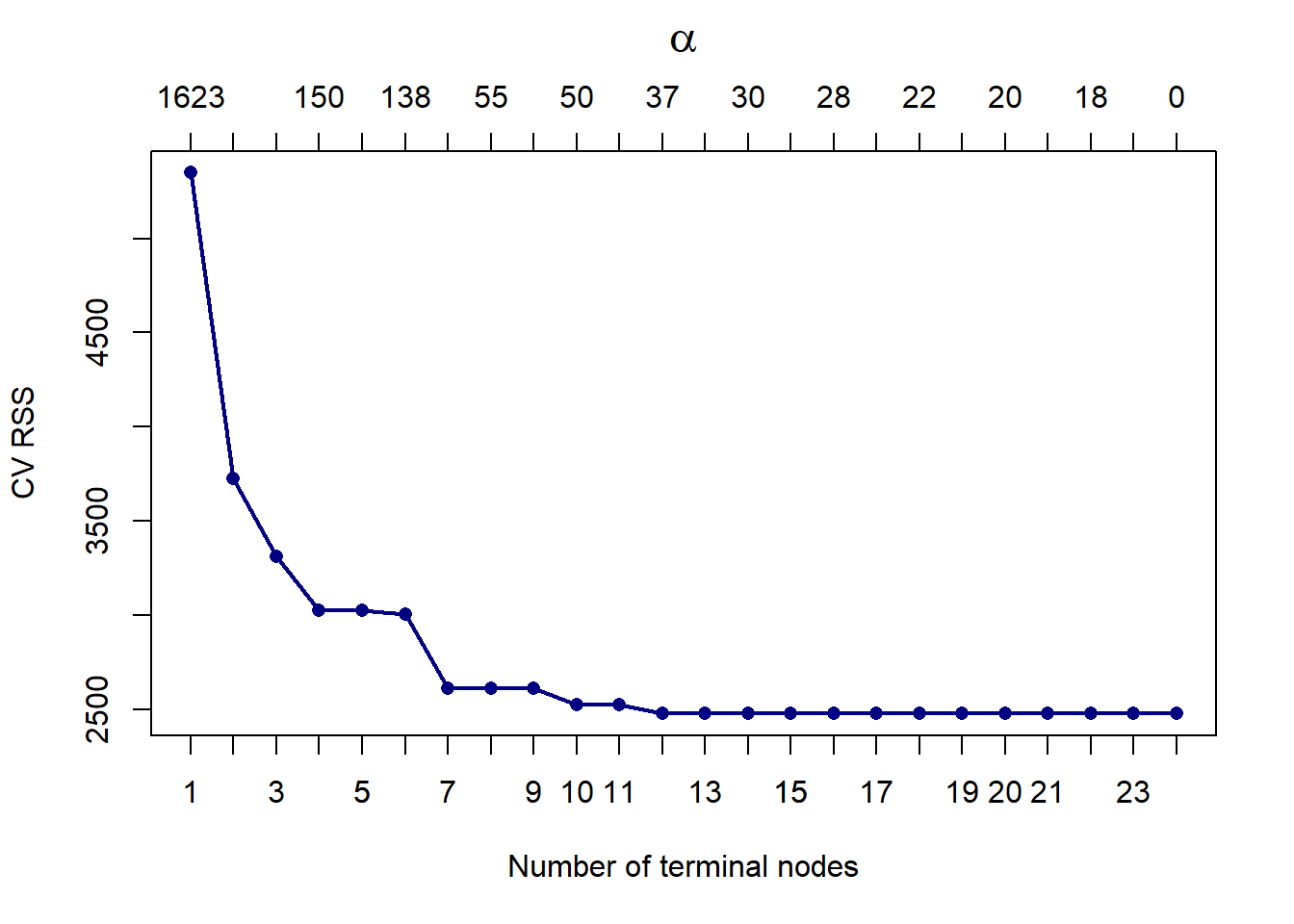
Figure 6.29: Cross-validated pruning results from a tree fitted to the feature-engineered Cailfornia housing training set.
The CV RSS first reaches a minimum at 12 terminal nodes, hence we will prune it down to that size.
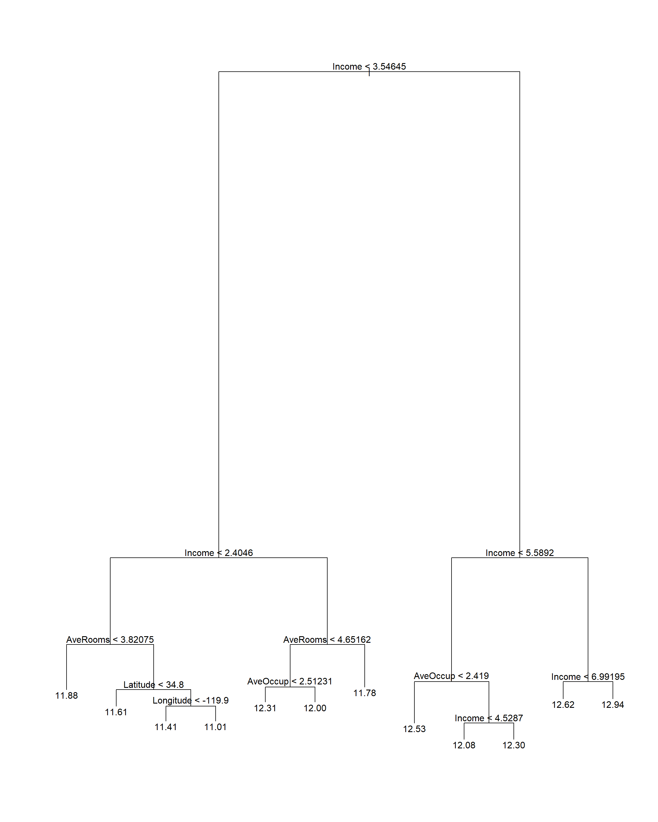
Figure 6.30: Pruning tree fitted to the feature-engineered Cailfornia housing training set.
Here we see that the average number of rooms and average occupancy were indeed useful in this model (compare to Figure 6.7, which split almost exclusively on income and location). The CV RMSE is 0.387.
Next, we fit a gradient boosted trees model to the training set via the gbm package, using caret to apply hyperparameter tuning according to 10-fold CV (which can be parallelised). Note that for a problem of this size, the gbm model does take a while to run. Therefore, the code run below has been commented out after running, with the results saved and loaded back in for quick reproducibility.
# set.seed(4026)
# ctrl <- trainControl(method = 'cv', number = 10, verboseIter = T)
#
# calif_gbm_grid <- expand.grid(n.trees = c(1000, 10000, 50000),
#                               interaction.depth = c(1, 2, 5),
#                               shrinkage = c(0.01, 0.001),
#                               n.minobsinnode = 10)
#
# calif_gbm_gridsearch <- train(HousePrice ~ ., data = calif_fe_train,
#                               method = 'gbm',
#                               distribution = 'gaussian',
#                               trControl = ctrl,
#                               verbose = T,
#                               tuneGrid = calif_gbm_grid)
# save(calif_gbm_gridsearch, file = 'data/gbm_calif_50k.Rdata')
load('data/gbm_calif_50k.Rdata')
Although we only touch on the subject here, the hyperparameter tuning procedure can be an entire topic on its own. One alternative to the grid search applied above – whereby all combinations of fixed sets of hyperparameter values are used – is to apply a random search, which introduces some variation in the hyperparameters. Bergstra & Bengio (2012) initially provided a strong argument for this approach within a neural network context. Further exploration of these topics is left for the reader.
Looking at the CV results in Figure 6.31, we see that higher values of \(d\) in fact yielded better results. As expected, the higher learning rate reduced the CV error quicker for the same number of trees.
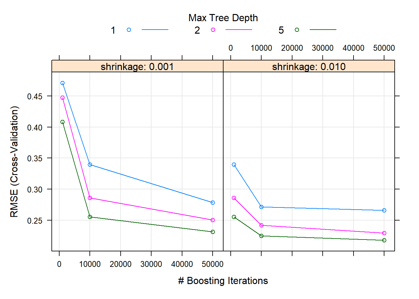
Figure 6.31: Hyperparameter combinations results for a gradient boosted trees model fitted to the feature-engineered California housing dataset.
However, it is important to note that for this particular combination of number of trees it is difficult to determine whether the error is still decreasing at 50,000 trees. One approach, as we will see later, is to apply early stopping, where training stops once improvement has ceased according to some specified condition. To explore this model’s behaviour, let’s use a large number of trees together with the best combination of \(\lambda\) and \(d\) from the grid search and see where the CV error reaches a minimum (Figure 6.32).
# calif_fe_gbm <-   gbm(HousePrice ~ ., data = calif_fe_train,
#                       distribution = 'gaussian',
#                       n.trees = 100000,
#                       interaction.depth = calif_gbm_gridsearch$bestTune$interaction.depth,
#                       shrinkage = calif_gbm_gridsearch$bestTune$shrinkage,
#                       bag.fraction = 1,
#                       cv.folds = 10,  #built-in CV
#                       n.cores = 10,   #which can be parallelised
#                       verbose = T)
# save(calif_fe_gbm, file = 'data/gbm_calif_100k.Rdata')
load('data/gbm_calif_100k.Rdata')
d <- gbm.perf(calif_fe_gbm)
legend('topright', c('CV error', 'Training error'), col = c('green', 'black'), lty = 1)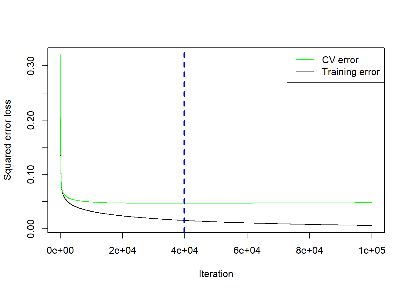
Figure 6.32: Cross-validation results for the gradient boosted trees model with \(\lambda=0.01\) and \(d=5\) fitted to the feature-engineered California housing dataset.
It turns out the CV error actually started increasing after 39731 trees. However, it is possible that one of the other hyperparameter combinations (different \(\lambda\) and \(d\)) would have yielded a lower CV if allowed to run for more than 50,000 trees. This example serves to illustrate that this style of hyperparameter tuning can be tedious, time-consuming, and a trial-and-error process. Although more sophisticated tuning techniques exist, such as random search and Bayesian optimisation, each has their own compromises and drawbacks. These are beyond the scope of this course.
The variable importance plots (this time using vi_permute()) are shown in Figure 6.33:
set.seed(1)

x_train <- select(calif_fe_train, -HousePrice)
y_train <- calif_fe_train$HousePrice

cgbm_pred_wrapper <- function(object, newdata) {
  predict(object, newdata = newdata, n.trees = d)  # d = chosen number of trees above
}

# cgbm_per_imp <- vi_permute(
#   object        = calif_fe_gbm,
#   feature_names = colnames(x_train),
#   train         = x_train,
#   target        = y_train,
#   metric        = 'rmse',
#   pred_wrapper  = cgbm_pred_wrapper,
#   nsim          = 5
# )
# save(cgbm_per_imp, file = 'data/calif_fe_perm_varimp.RData')
load('data/calif_fe_perm_varimp.RData')

cgbm_per_p <- vip(cgbm_per_imp) +
  labs(
    title = 'Permutation Variable Importance',
    x = 'Increase in Prediction Error',
    y = NULL
  ) +
  theme_minimal()

cgbm_imp_p <- vip(calif_fe_gbm) +
  labs(
    title = 'Impurity Variable Importance',
    x = 'Decrease in Splitting Criterion',
    y = NULL
  ) +
  theme_minimal()

cgbm_per_p + cgbm_imp_p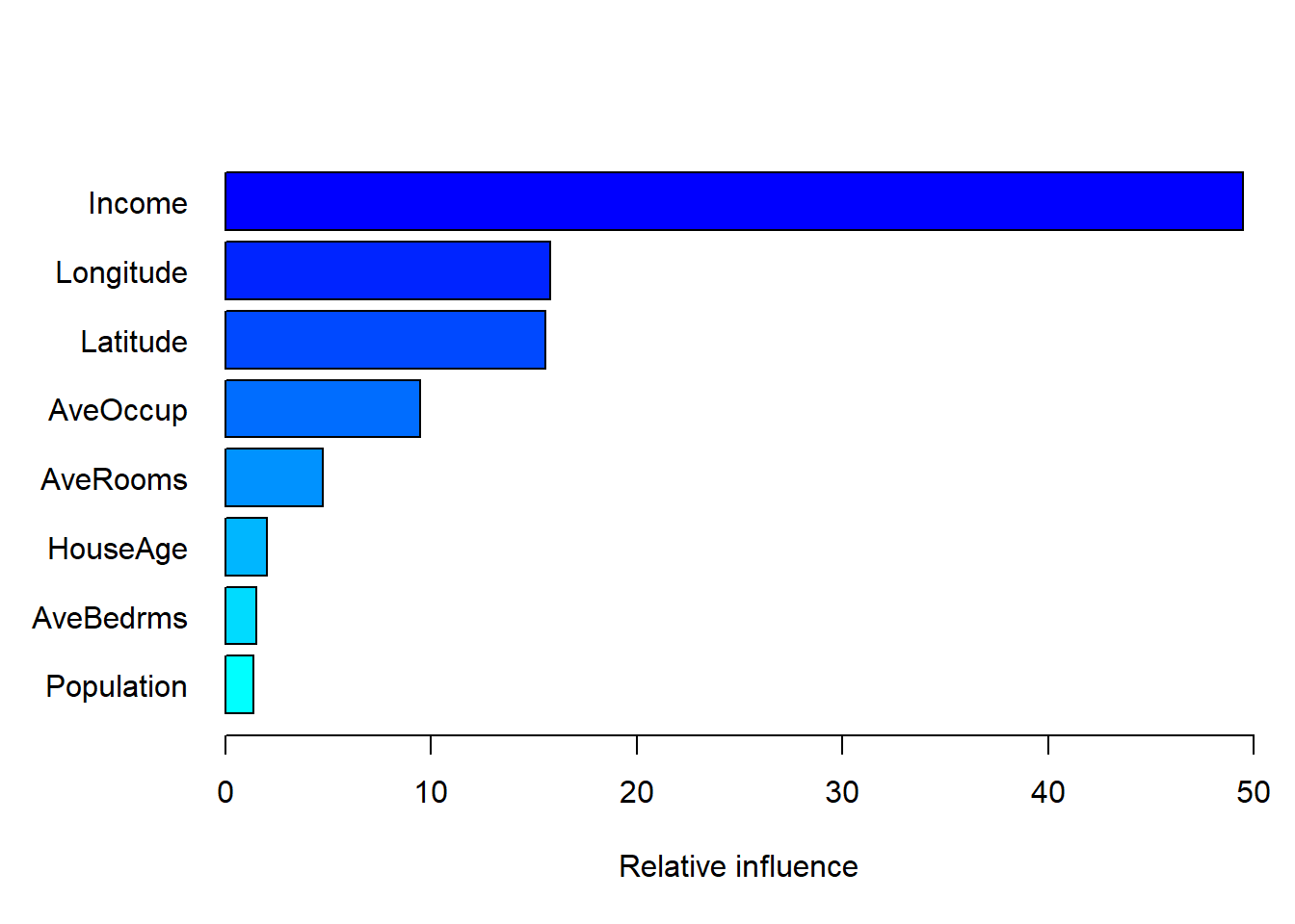
Figure 6.33: Variable importance for the tuned gbm model fitted to the feature-engineered California housing dataset.
We see that according to impurity-based importance, Income appears dominant, implying that it is highly effective at reducing training RSS and is frequently used in early splits. Permutation-based importance, on the other hand, reflects the extent to which the model’s predictive performance depends uniquely on a variable. Since Income is strongly correlated with the spatial predictors Latitude and Longitude, permuting it does not degrade predictive accuracy as dramatically as its split-based contribution might suggest. This highlights that impurity importance measures how much a variable is used in constructing the model, whereas permutation importance measures how much the model relies on that variable for prediction.
It’s also worth noting that two of our engineered features – average occupancy and average rooms – were somewhat influential according to both measures.
Although variable importance plots tell us which features are most important for predicting the response, they do not tell us how the predictors influence the predictions. A number of model-agnostic methods have been developed to quantify and explore the contribution of features to model predictions. These include Partial Dependence Plots, Individual Conditional Expectation (ICE) curves, Accumulated Local Effects (ALE) plots, and Shapley value–based methods (often referred to as SHAP). Whereas variable importance provides a global ranking of predictors, these approaches aim to characterise how predictions change as a function of specific features. Molnar (2020) provides a comprehensive overview of Interpretable Machine Learning, with the book freely accessible here.
Shapley methods in particular have become popular in modern machine learning. Rooted in cooperative game theory, Shapley values attribute to each feature its average marginal contribution to the prediction across all possible coalitions of predictors. This provides a theoretically principled decomposition of individual predictions, but at the cost of additional computational and conceptual complexity.
For reasons of scope, we restrict attention here to Partial Dependence Plots, which provide a simple and intuitive way to visualise the marginal relationship between a predictor and the fitted response. While PDPs are not without limitations – particularly in the presence of correlated predictors – they remain a useful entry point into model interpretation.
6.4.2 Partial dependence plots
Partial dependence functions can be used to interpret the results of any “black box” learning method by measuring the relationship between certain features and the approximation of \(f(\boldsymbol{X})\). For \(p\) features, \(X_1, \ldots, X_p\), consider some feature \(X_j\) and let \(X_{-j}\) denote all other features.
One way to define the average or partial dependence of \(f(\boldsymbol{X})\) on \(X_j\) is
\[f_j(X_j) = E_{X_{-j}}f(X_j, X_{-j}),\]
which can be estimated by
\[\bar{f}_j(X_j) =\frac{1}{N} \sum_{i=1}^N f(X_j, X_{i,-j}).\] This must be done for each value of \(X_j\) and can be computationally intensive, even for moderately-sized datasets. Note that these partial dependence functions represent the effect of \(X_j\) on \(f(\boldsymbol{X})\) after accounting for the average effects of the other features on \(f(\boldsymbol{X})\), as opposed to the effect of \(X_j\) on \(f(\boldsymbol{X})\) when ignoring the effects of the \(X_{-j}\).
Unfortunately, visualisation of these relationships is limited to low-dimensional views. Although these “slices” of information can seldom provide a comprehensive depiction of the approximation, it can still provide a useful indication of how certain features influenced the predictions on average, especially when their interaction with other variables is limited.
The gbm package again allows us to easily produce the partial dependence plots. Figure 6.34 shows 1-dimensional partial dependence plots for the previously fitted model on the (feature-engineered) California dataset for four of the (non-location) features.
library(gridExtra)
library(grid)

ylims <- c(11.5,12.8)
p1 <- plot.gbm(calif_fe_gbm, 'Income', d, ylim = ylims, ylab = '')
p2 <- plot.gbm(calif_fe_gbm, 'AveRooms', d, ylim = ylims, ylab = '', xlab = 'Average Rooms')
p3 <- plot.gbm(calif_fe_gbm, 'AveOccup', d, ylim = ylims, ylab = '', xlab = 'Average Occupancy')
p4 <- plot.gbm(calif_fe_gbm, 'HouseAge', d, ylim = ylims, ylab = '', xlab = 'House Age')

grid.arrange(p1, p2, p3, p4, ncol = 2)
grid.text('Partial Predicted Log House Price', x = 0, vjust = 1, rot = 90)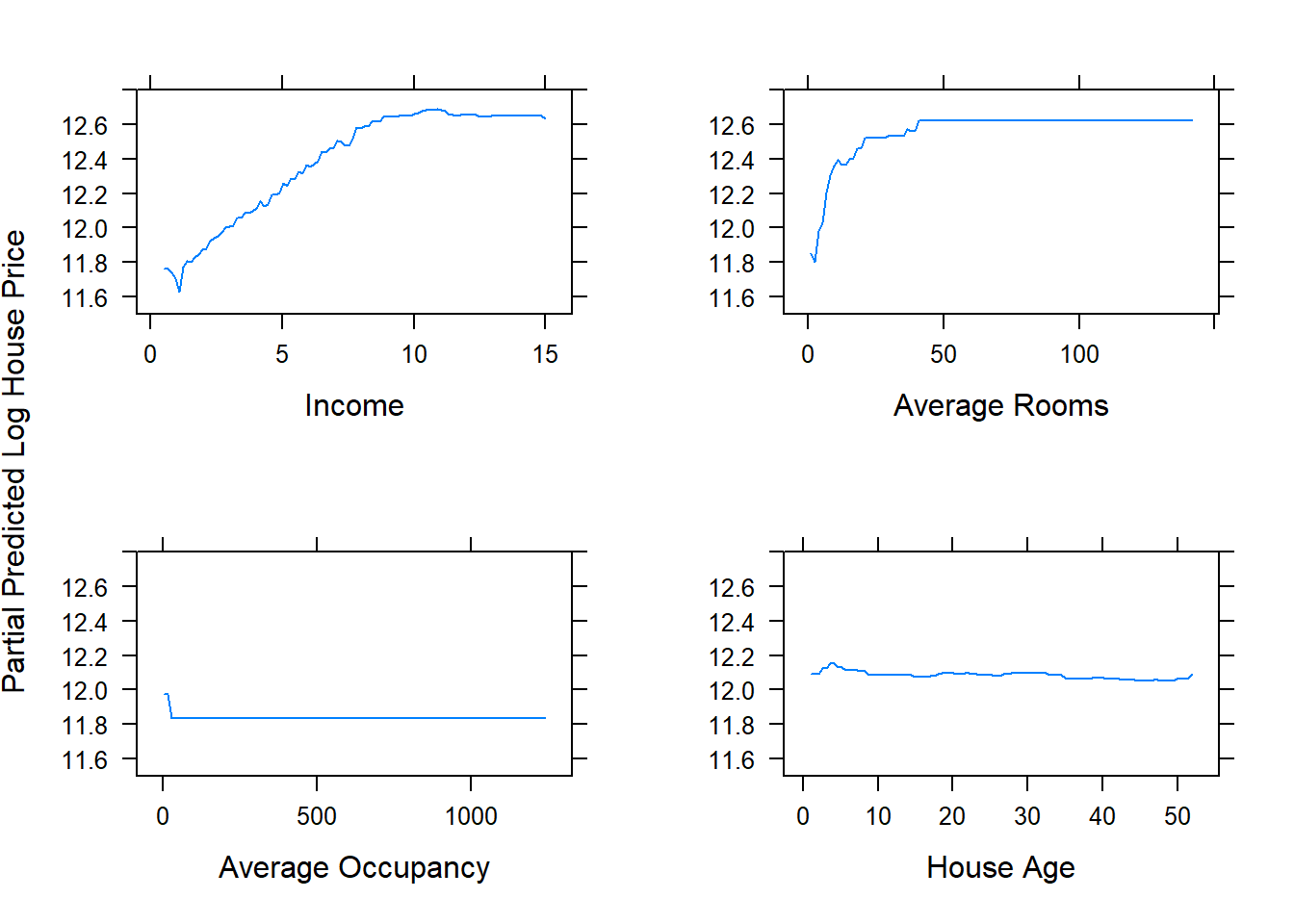
Figure 6.34: Partial dependence plots for the gbm model fitted to the feature-engineered California housing dataset.
Looking at the average occupancy and average rooms, something is not right – an average occupancy of more than 1000 does not make sense, nor does more than 100 rooms on average! It is most likely an errant observation(s) with too few households.
##       HousePrice  Income HouseAge Rooms Bedrooms Population Households Latitude Longitude
## 19007 11.83138 10.2264 45 19 5 7460 6 38.32 -121.98## HousePrice Income HouseAge Rooms Bedrooms Population Households Latitude Longitude
## 1915 13.12237 1.875 33 1561 282 30 11 38.91 -120.1Indeed, six households for a population of 7460 is nonsensical. 1561 rooms for 11 households and a population of 30 is questionable, given some of the areas filled with mansions one finds in California. This goes to show how important an exploratory data analysis and cleaning are at the start of an analysis! These are just the observations yielding the maximum average occupancy and average rooms values, one could explore their distributions further.
It would be best to rerun the analysis with the cleaned data, which is left as a homework exercise. For now, we will just cut off these outliers, for which we can use a package offering more options for partial dependence plots. pdp is a popular package for this.
library(pdp)

p1 <- pdp::partial(calif_fe_gbm, 'Income',   n.trees = d)
p2 <- pdp::partial(calif_fe_gbm, 'AveRooms', n.trees = d, trim.outliers = T)
p3 <- pdp::partial(calif_fe_gbm, 'AveOccup', n.trees = d, trim.outliers = T)
p4 <- pdp::partial(calif_fe_gbm, 'HouseAge', n.trees = d)

grid.arrange(plotPartial(p1, ylab = '', ylim = ylims),
             plotPartial(p2, ylab = '', ylim = ylims, xlab = 'Average Rooms'),
             plotPartial(p3, ylab = '', ylim = ylims, xlab = 'Average Occupancy'),
             plotPartial(p4, ylab = '', ylim = ylims, xlab = 'House Age'),
             ncol = 2)
grid.text('Partial Predicted Log House Price', x = 0, vjust = 1, rot = 90)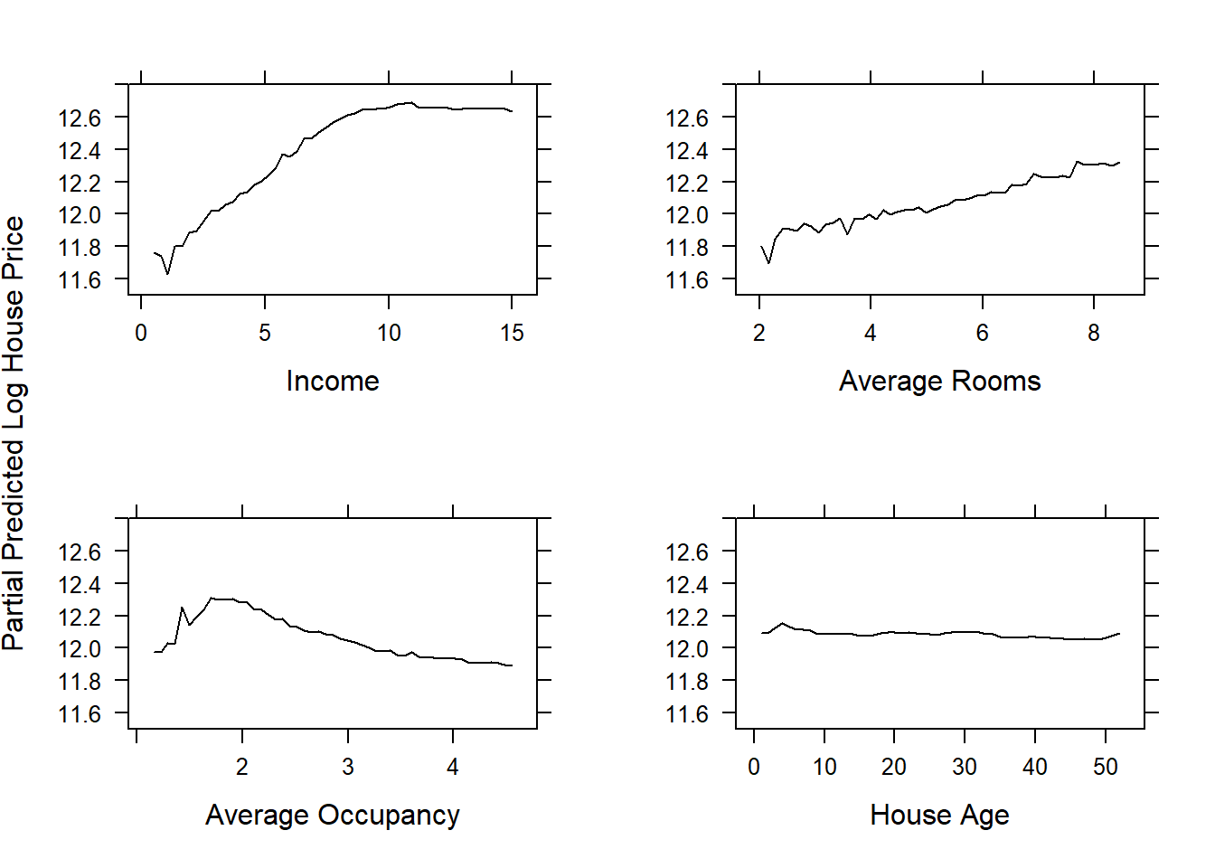
Figure 6.35: Partial dependence plots for some of the features in the gbm model fitted to the feature-engineered California housing dataset. Some of the x-axes have been rescaled.
The lack of discernible relationship between house age and predicted house price reflects its low variable importance, noting that the y-axes have been adjusted such that the features are directly comparable. For income and average rooms we observe a general positive relationship, whilst increasing average occupancy initially increases the predicted house price (although increasing the resolution could add a lot of noise between one and two occupants), before it gradually decreases.
Finally, we can also look at the partial dependence of two features simultaneously. To come full-circle with this example, we will do so for the latitude and longitude. In order to add the map border, we will extract the partial dependence information.
latlong_pd <- plot.gbm(calif_fe_gbm, c('Longitude', 'Latitude'), return.grid = T)

# Same colour scale as before
n_breaks <- 9
my_cols <- brewer.pal(n_breaks, 'YlOrBr')[cut(latlong_pd$y, breaks = n_breaks)]

# Plot the partial dependence values
plot(latlong_pd$Longitude, latlong_pd$Latitude, pch = 15,
     xlab = 'Longitude', ylab = 'Latitude', col = my_cols)
legend(x = 'topright', bty = 'n', title = 'Log Median House Price', cex = 0.9,
       legend = round(seq(min(latlong_pd$y), max(latlong_pd$y), length.out = n_breaks), 2),
       fill = brewer.pal(n_breaks, 'YlOrBr'))

# Add the state border
par(new = TRUE)
map('state', 'california', add = T, lwd = 2) |> invisible()
text(-123, 35, 'Pacific Ocean')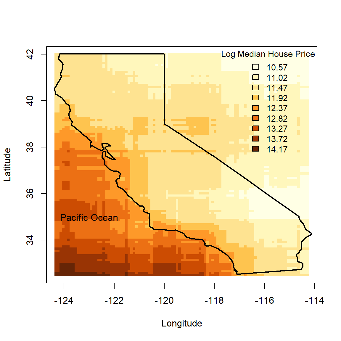
Figure 6.36: Partial dependence plot of the location information for the gbm model fitted to the feature-engineered California housing dataset.
In Figure 6.36 we see that the model extrapolates beyond the state boundaries, extending the general trend observed earlier of “the more south-west, the more expensive”. This completely messes up the colour scale, so to get a more realistic and useful picture let us rather only plot the partial dependence information pertaining to populated locations.
library(latticeExtra)

locs <- distinct(calif, Longitude, Latitude)
p <- pdp::partial(calif_fe_gbm, c('Longitude', 'Latitude'), locs, n.trees = d)

# Same colour scale as before
n_breaks <- 9
my_cols <- colorRampPalette(brewer.pal(n_breaks, 'YlOrBr'))

pp <- plotPartial(p, col.regions = my_cols(100))

# Add the state border. plotPartial creates a lattice be default
my_map <- map_data('state', 'california')
border_layer <- latticeExtra::layer(panel.polygon(my_map, col = 'transparent'))
pp + border_layer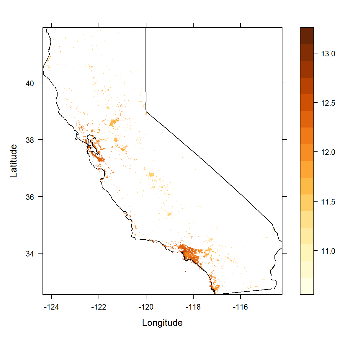
Figure 6.37: Partial dependence plot for the observed location information for the gbm model fitted to the feature-engineered California housing dataset.
Comparing this with Figure 6.1, we can see how the gbm model learned how location relates to house price.
So far we have only discussed the base version of stochastic gradient boosting, but there are many variants that use the same basic principle whilst making changes to some aspects of the algorithm. One particularly powerful, relatively recent development is Extreme Gradient Boosting (XGBoost).
6.4.3 XGBoost
Since Chen & Guestrin (2016) first proposed XGBoost, it has become one of the most widely used algorithms for supervised learning on structured (tabular) data. Conceptually, it is a gradient boosting method built from regression trees, but with several important refinements that improve statistical regularisation and computational efficiency. For the sake of scope we summarise the key innovations below.
Explicit regularised objective:
XGBoost minimises a regularised objective function of the form
\[\sum_{i=1}^n \ell(y_i, \hat y_i) + \sum_{m=1}^M \left( \gamma J_m + \frac{\lambda}{2} \sum_{j=1}^{J_m} w_{jm}^2 \right),\] where \(J_m\) is the number of leaves in tree \(m\) and \(w_{jm}\) are the leaf weights. The parameters \(\gamma\), \(\lambda\) (and optionally an \(L_1\) penalty) explicitly control tree complexity and shrink leaf predictions, reducing overfitting.Second-order (Newton) boosting:
Rather than using only first-order gradients, XGBoost employs a second-order Taylor expansion of the loss function. This incorporates both gradients and Hessians when computing optimal leaf weights, leading to more stable and often faster convergence.Shrinkage and stochastic regularisation:
In addition to the learning rate \(\eta\), XGBoost supports row subsampling (subsample) and column subsampling (colsample_bytree, etc.). These introduce randomness across boosting iterations, reducing variance and improving generalisation.Greedy tree construction with pruning:
Trees are grown using a gain-based splitting criterion derived from the regularised objective. Splits that do not achieve sufficient improvement (controlled by \(\gamma\)) are discarded, effectively pruning the tree.Handling of missing values:
During training, XGBoost learns the optimal default direction (left or right) for observations with missing values at each split. This allows missingness to be handled internally without prior imputation.Computational efficiency:
The algorithm is designed for parallelisation and efficient memory usage, enabling large-scale training on modern hardware.
XGBoost can, therefore, be viewed as a regularised, second-order extension of classical gradient boosting, combining statistical shrinkage and structural constraints with computational refinements to yield a highly effective and scalable tree-based learner.
We will now analyse the California data one final time using the xgboost package. In earlier versions, it was convenient to tune XGBoost via caret::train(method = "xgbTree"). However, at time of writing, recent xgboost releases introduced breaking changes in the underlying R objects that can cause caret fits/tuning to fail.
Although other modelling and tuning frameworks exist (see Section 6.4.5 at the end), each has its own quirks and syntax to learn. We can, however, use XGBoost’s built-in CV grid search tuning function – xgb.cv() – which also applies early stopping. The only additional requirement is that the data be transformed into an “xgb.DMatrix” object.
For illustration purposes we will search over:
- tree depth \(d\in\{6, 8\}\)
- learning rate \(\eta\in\{0.005, 0.01\}\)
- feature subsampling per tree \(\in\{0.5, 1\}\)
- row subsampling per tree \(\in\{0.5, 1\}\)
- L2 penalty on the leaf weights \(\lambda \in \{0.5, 1, 5\}\)
We allow up to 40,000 trees, but early stopping will terminate the training if CV error does not decrease for \(k\) trees. We will set \(k = 200\).
library(xgboost)
library(purrr)
library(tibble)

# Design matrix for xgboost (one-hot encoding if needed)
x_train <- model.matrix(HousePrice ~ . - 1, data = calif_fe_train)
y_train <- calif_fe_train$HousePrice
dtrain  <- xgb.DMatrix(data = x_train, label = y_train)

# Hyperparameters
calif_xgb_grid <- expand.grid(
  max_depth        = c(6, 8),        #max interaction depth (d)
  eta              = c(0.01, 0.005), #learning rate
  colsample_bytree = c(0.5, 1),      #proportion of random features per tree
  subsample        = c(0.5, 1),      #proportion of training instances
  lambda           = c(0.5, 1, 5),   #L2 penalty on leaf weights
  gamma            = 0.001,          #mindev, also controls tree depth
  min_child_weight = 1               #also controls tree depth
)

set.seed(1)

# A manual collection of CV results
# calif_xgb_gridsearch <- pmap_dfr(calif_xgb_grid,
#                                  function(max_depth, eta, colsample_bytree, subsample, lambda, gamma, min_child_weight) {
#
#                                    params <- list(
#                                      booster          = 'gbtree',           #default
#                                      objective        = 'reg:squarederror', #training objective function
#                                      eval_metric      = 'rmse',             #CV performance measure
#                                      max_depth        = max_depth,
#                                      eta              = eta,
#                                      colsample_bytree = colsample_bytree,
#                                      subsample        = subsample,
#                                      lambda           = lambda,
#                                      gamma            = gamma,
#                                      min_child_weight = min_child_weight
#                                    )
#
#                                    cv <- xgb.cv(
#                                      params                = params,
#                                      data                  = dtrain,
#                                      nrounds               = 40000,
#                                      nfold                 = 5,
#                                      early_stopping_rounds = 200,
#                                      verbose               = 0
#                                    )
#
#                                    tibble(
#                                      max_depth        = max_depth,
#                                      eta              = eta,
#                                      colsample_bytree = colsample_bytree,
#                                      subsample        = subsample,
#                                      lambda           = lambda,
#                                      ntrees           = cv$early_stop$best_iteration,
#                                      rmse             = cv$early_stop$best_score
#                                    )
#                                  }
# )
#
# save(calif_xgb_gridsearch, file = 'data/xgb_calif.RData')
load('data/xgb_calif.RData')
best <- calif_xgb_gridsearch |> slice_min(rmse, n = 1)
Plotting the grid search CV results across so many hyperparameter combinations is not sensible, even for this example where we only used two values for most of the HPs. Figure 6.38 shows only the best learning rate and depth combinations across all other HPs. Once again we see that shallower trees and lower learning rates require more iterations for the CV error to reach a minimum.
best_eta_depth <- calif_xgb_gridsearch %>%
  group_by(eta, max_depth) %>%
  slice_min(rmse, n = 1, with_ties = FALSE) %>%
  ungroup()

ggplot(best_eta_depth,
       aes(x = ntrees,
           y = rmse,
           colour = factor(max_depth),
           shape = factor(eta),
           group = interaction(max_depth, eta))) +
  geom_point(size = 2) +
  labs(
    x = 'Number of trees (best iteration)',
    y = 'CV RMSE',
    colour = 'Max depth (d)',
    shape = 'Learning rate (eta)'
  ) +
  theme_minimal()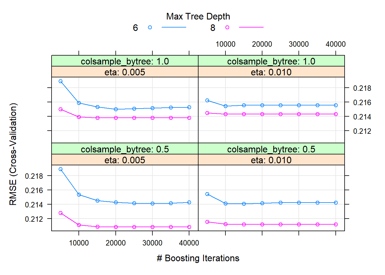
Figure 6.38: Hyperparameter grid search results for XGBoost fitted to the feature-engineered California housing dataset using xgboost::xgb.cv with early stopping. Each point is the best learning rate and depth combination across all other hyperparameters.
The overall best combination (of the ones tested) is:
| max_depth | eta | colsample_bytree | subsample | lambda | ntrees | rmse |
|---|---|---|---|---|---|---|
| 8 | 0.005 | 0.5 | 0.5 | 0.5 | 8580 | 0.2110014 |
Once the best hyperparameter combination is selected, we fit a final model using the corresponding optimal number of trees (best_iteration) and evaluate it on the test set.
calif_fe_xtest <- model.matrix(HousePrice ~ . - 1, data = calif_fe_test)
calif_fe_ytest <- calif_fe_test$HousePrice

params_best <- list(
  booster          = 'gbtree',
  objective        = 'reg:squarederror',
  eval_metric      = 'rmse',
  max_depth        = best$max_depth,
  eta              = best$eta,
  colsample_bytree = best$colsample_bytree,
  subsample        = best$subsample,
  lambda           = best$lambda,
  gamma            = 0.001,
  min_child_weight = 1
)

set.seed(1)
calif_xgb <- xgb.train(
  params  = params_best,
  data    = dtrain,
  nrounds = best$ntrees,
  verbose = 0
)

calif_xgb_pred <- predict(calif_xgb, newdata = calif_fe_xtest)
calif_xgb_rmse <- mean((calif_fe_ytest - calif_xgb_pred)^2) |> sqrt()
The CV RMSE of 0.211 was relatively close to the testing RMSE of 0.208, in fact slightly overestimating it. We can also determine the proportion of variation explained in the unseen data as \(R^2\) = 86.61%.
One way of visualising a model’s predictions is to simply plot them against the observed values. The closer the points lie to a straight line, the better the fit.
plot_data <- as.data.frame(cbind(predicted = calif_xgb_pred, observed = calif_fe_test$HousePrice))

ggplot(plot_data, aes(predicted, observed)) + geom_point(color = 'darkred', alpha = 0.5) +
  geom_smooth(method = lm) +
  xlab('Predicted log(price)') + ylab('Observed log(price)') +
  theme(plot.title = element_text(color = 'darkgreen', size = 16, hjust = 0.5),
        axis.text.y = element_text(size = 12), axis.text.x = element_text(size = 12, hjust = 0.5),
        axis.title.x = element_text(size = 14), axis.title.y = element_text(size = 14)) +
  theme_bw()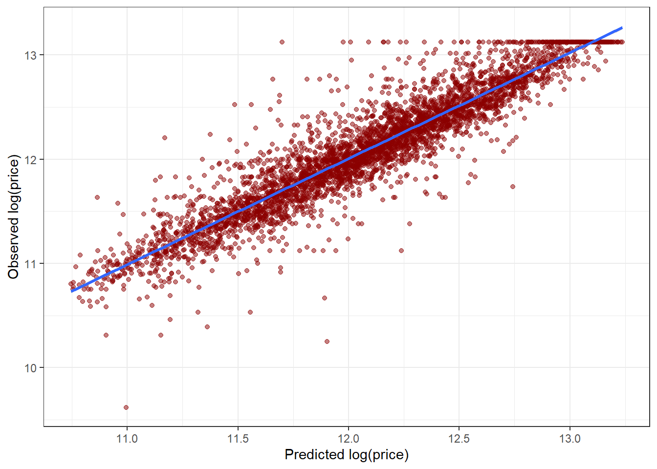
The first thing to notice is the clear ceiling on the observed house prices, which one should once again ideally have already picked up in the data exploration. This maximum value of 500001 is suspiciously round. It turns out that there are 992 neighbourhoods where the median house price was either $500,000 or $500,001. Whether this is an artifact of the data due to some measurement limit or estimation, or whether it was because of some real-world bound is something the analyst should determine before providing definitive conclusions.
For our very last example, we will return to the Titanic data.
6.4.4 Example 7 – Titanic (continued)
Slow learning methods like gradient boosting generally tend to work better on larger datasets. Having said that, nothing prevents us from applying boosting to the Titanic data for comparison, even though it is relatively limited in size.
The benefit of a smaller problem is of course that the training goes quicker and it generally requires fewer trees, such that one can test more hyperparameter combinations for the same time cost. Subsampling is also unlikely to yield much, if any benefit, hence we will just use the gbm method.
We will search across trees from 500 to 6000 in increments of 500; \(d = 1, \ldots, 5\); and \(\lambda \in (0.001, 0.005, 0.01)\).
set.seed(1)
train <- sample(1:nrow(titanic), 0.7*nrow(titanic))

titanic_train <- titanic[train,]
titanic_test <- titanic[-train,]

# set.seed(4026)
# titanic_gbm_grid <- expand.grid(n.trees = seq(500, 6000, 500),
#                                 interaction.depth = 1:5,
#                                 shrinkage = c(0.01, 0.005, 0.001),
#                                 n.minobsinnode = 1)
#
# ctrl <-  trainControl(method = 'cv', number = 10, verboseIter = T)
#
# titanic_gbm_gridsearch <- train(Survived ~ ., data = titanic_train,
#                                 method = 'gbm',
#                                 distribution = 'bernoulli', #For classification
#                                 trControl = ctrl,
#                                 verbose = F,
#                                 tuneGrid = titanic_gbm_grid)
# save(titanic_gbm_gridsearch, file = 'data/gbm_titanic.Rdata')
load('data/gbm_titanic.Rdata')
Viewing the hyperparameter tuning results:
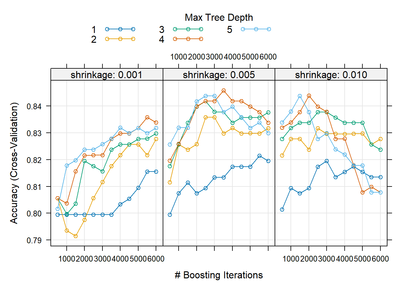
Figure 6.39: Hyperparameter combinations results for a gradient boosted trees model fitted to the Titanic dataset.
The best model used the following hyperparameters:
| n.trees | interaction.depth | shrinkage | n.minobsinnode | |
|---|---|---|---|---|
| 103 | 3500 | 4 | 0.005 | 1 |
This is a desirable result, since none of the hyperparameters are on the edge of the explored space. Using \(d = 4\) and \(\lambda = 0.005\), we can now find the exact number of trees where the CV deviance is minimised.
# gbm requires 0-1 for binary classification (without caret)
titanic_train$Survived <- as.numeric(titanic_train$Survived) - 1

set.seed(4026)
titanic_gbm <- gbm(Survived ~ ., data = titanic_train,
                   distribution = 'bernoulli',    #For binary classification (see ?gbm)
                   n.trees = titanic_gbm_gridsearch$bestTune$n.trees,
                   interaction.depth = titanic_gbm_gridsearch$bestTune$interaction.depth,
                   shrinkage = titanic_gbm_gridsearch$bestTune$shrinkage,
                   n.minobsinnode = titanic_gbm_gridsearch$bestTune$n.minobsinnode,
                   bag.fraction = 1,
                   cv.folds = 10,
                   n.cores = 10,
                   verbose = F)

d <- gbm.perf(titanic_gbm)
legend('topright', c('CV error', 'Training error'), col = c('green', 'black'), lty = 1)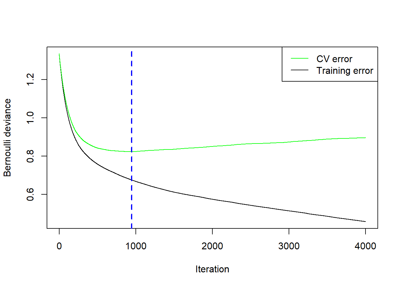
Figure 6.40: Cross-validation results for the gradient boosted trees model with \(\lambda=0.005\) and \(d=4\) fitted to the Titanic dataset.
We will use this model, with only 1103 trees, for prediction.
y_titanic_test <- as.numeric(titanic_test$Survived) - 1
titanic_gbm_pred <- predict(titanic_gbm, newdata = titanic_test, type = 'response')
titanic_gbm_mis <- mean(y_titanic_test != round(titanic_gbm_pred))
Through gbm we have managed to reduce the testing misclassification rate even further, from 21.4% for the tuned random forest to 21.86%. Exploring the confusion matrix and other classification metrics is left as an exercise.
According to this model, passenger sex is still the most influential predictor. Age and passenger follow with similar levels of contribution. It’s worth noting that the impurity and permutation variable importance measures are quite similar, contrary to the random forest model variable importance shown in Figure 6.28, where passenger class contributed relatively more to classification accuracy during prediction than it contributed during splitting.
set.seed(1)

x_train <- select(titanic_train, -Survived)
y_train <- titanic_train$Survived |> as.factor()

tgbm_pred_wrapper <- function(object, newdata) {
  p <- predict(object, newdata = newdata, n.trees = d, type = 'response')  # d = chosen number of trees above
  factor(as.integer(p >= 0.5), levels = levels(y_train))
}

#See vip::list_metrics() for a list of metrics

tgbm_per_imp <- vi_permute(
  object        = titanic_gbm,
  feature_names = colnames(x_train),
  train         = x_train,
  target        = y_train,
  metric        = 'accuracy',
  pred_wrapper  = tgbm_pred_wrapper,
  nsim          = 10
)

tgbm_per_p <- vip(tgbm_per_imp) +
  labs(
    title = 'Permutation Variable Importance',
    x = 'Increase in Prediction Error',
    y = NULL
  ) +
  theme_minimal()

tgbm_imp_p <- vip(titanic_gbm) +
  labs(
    title = 'Impurity Variable Importance',
    x = 'Decrease in Splitting Criterion',
    y = NULL
  ) +
  theme_minimal()

tgbm_per_p + tgbm_imp_p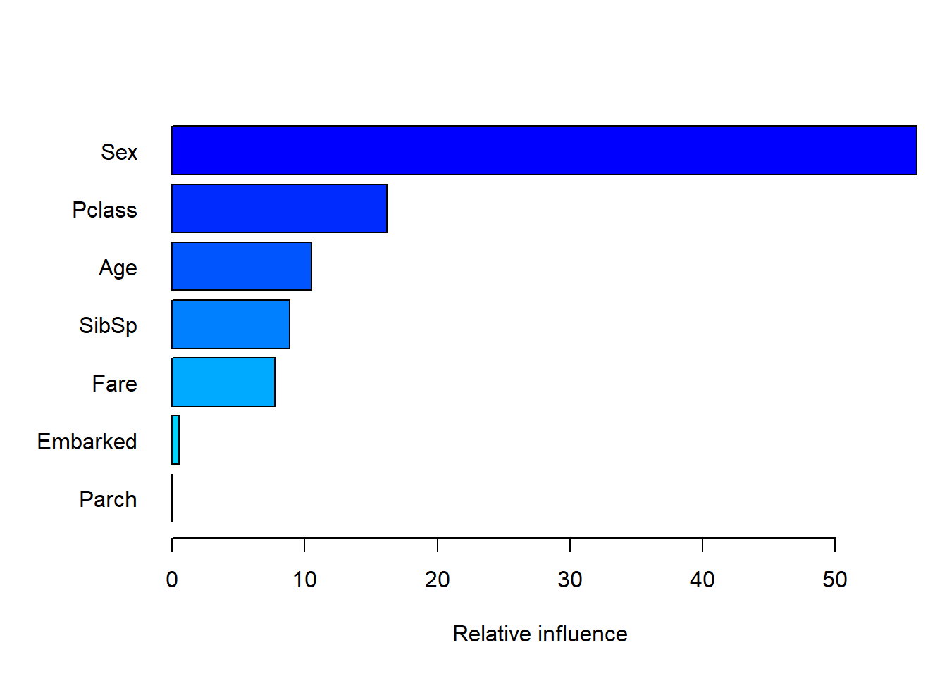
Figure 6.41: Variable importance for the tuned gbm model fitted to the Titanic dataset.
Moving on to the partial dependence plots, we observe the expected patterns based on the classification tree, where the log-odds of survival were significantly increased by being female; decreased as class increases; dipped sharply after late-teens, but picked up again for the elderly; and increased sharply beyond a specific fare. There are once again outliers in fare which can be removed, although this is left for the reader.
p1 <- plot.gbm(titanic_gbm, 'Sex', d, ylab = '', type = 'response', ylim = c(0,1))
p2 <- plot.gbm(titanic_gbm, 'Pclass', d, ylab = '', type = 'response', ylim = c(0,1))
p3 <- plot.gbm(titanic_gbm, 'Age', d, ylab = '', type = 'response', ylim = c(0,1))
p4 <- plot.gbm(titanic_gbm, 'Fare', d, ylab = '', type = 'response', ylim = c(0,1))

grid.arrange(p1, p2, p3, p4, ncol = 2)
grid.text('Partial Predicted Probability', x = 0, vjust = 1, rot = 90)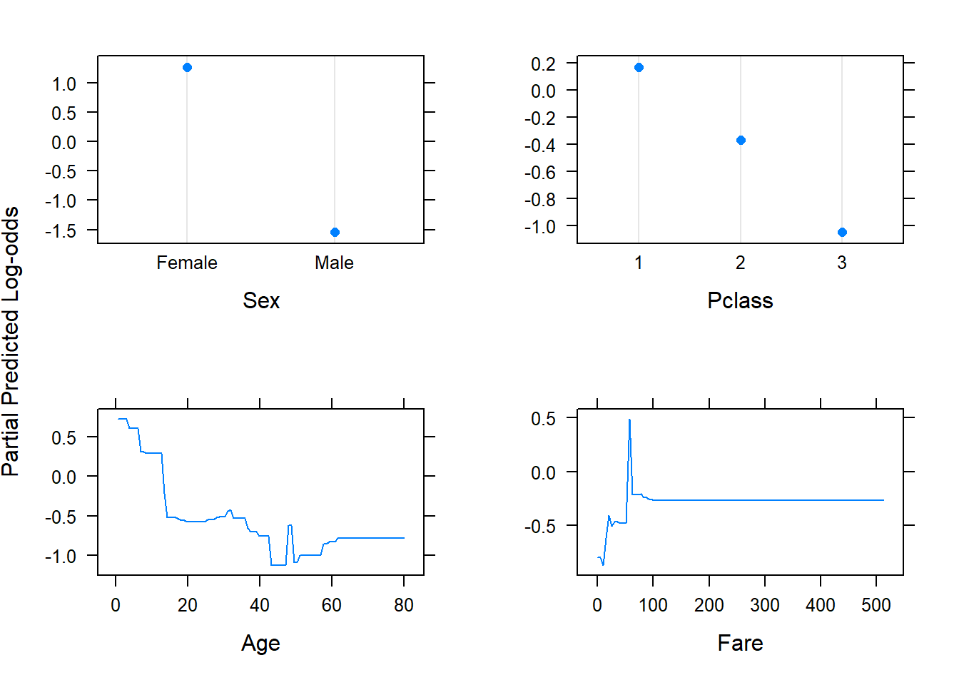
Figure 6.42: Partial dependence plots for the gbm model fitted to the Titanic dataset.
We might also be interested in the interaction between age and sex, shown in Figure 6.43.
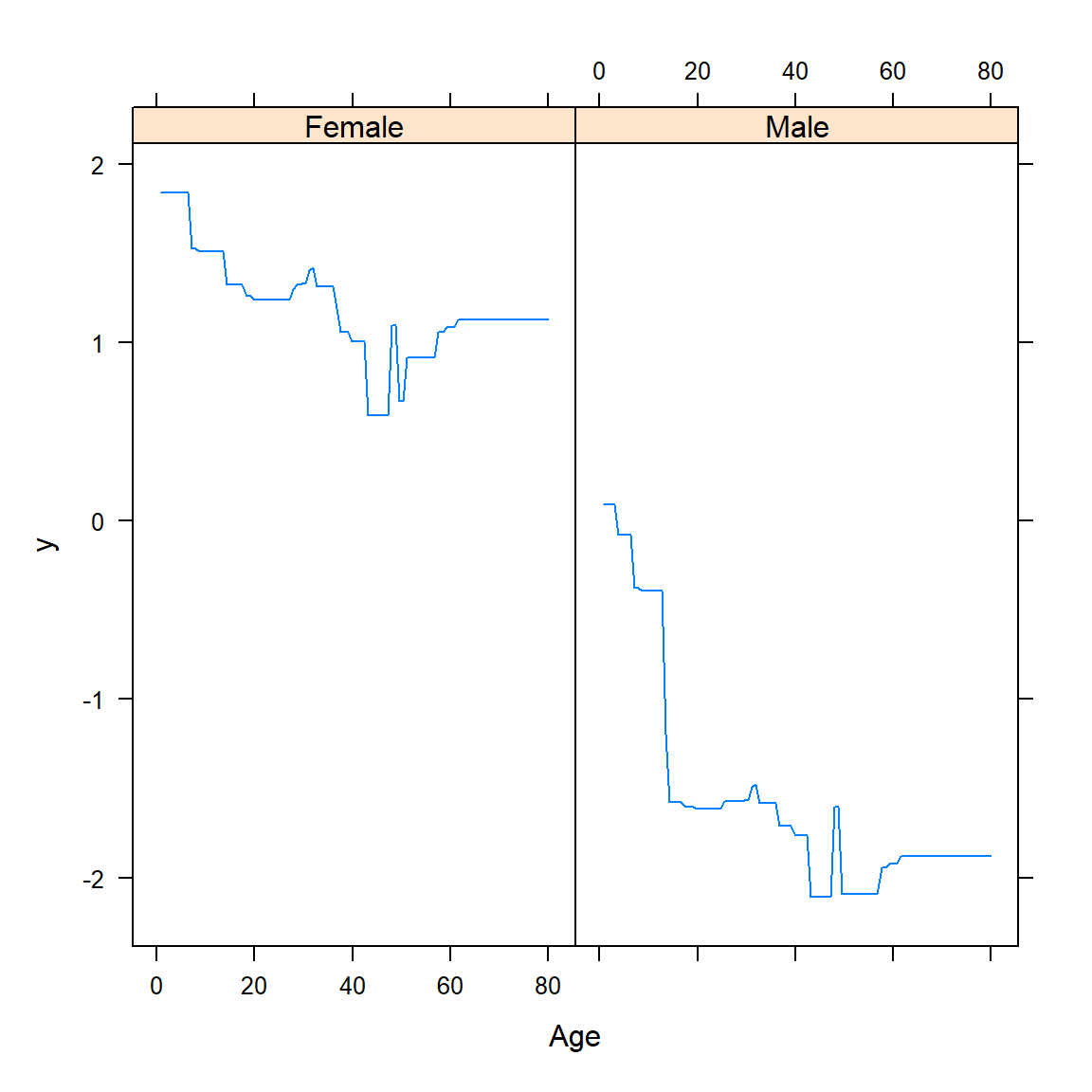
Figure 6.43: Bivariate partial dependence plot for the gbm model fitted to the Titanic dataset.
Although the overall pattern across ages is roughly the same for males and females, we do a see a noticeably more pronounced dip specifically for males beyond age of approximately 16.
These various approaches have allowed us to extract useful insights into the data (statistical learning paradigm) as well create some relatively accurate predictions on unseen data (machine learning paradigm).
6.4.5 Final word
We end this section with one final reminder that the implementation of these supervised learning algorithms is constantly being developed. For example, we mostly used caret for hyperparameter tuning, although one could achieve the same with a number of other libraries, e.g. the now widely-used tidymodels framework, or the more powerful (but less convenient) mlr3 package.
You are encouraged to keep on exploring new methods in R, although one should always ensure that you have a deeply grounded understanding of the theory underpinning these methods. So continue balancing depth of theory, breadth of topic, and practical application on your future journey through supervised learning.
Happy continued learning!
6.5 Homework exercises
We observed a fairly high \(R^2\) value for the random forest fitted to the California housing dataset. How does this compare to the other regression models we encountered? Compare it with the lasso regression, some polynomial regression model, and KNN.
Run the random forest grid search on the Titanic dataset multiple times. What is the distribution of hyperparameter selections? How does the splitting rule choice affect the predictive performance and variable importance measurements?
Rerun the feature-engineered California housing analyses after removing all definite outliers. Does this affect any of the results?
Fit and tune a random forest on the feature-engineered California training set. How do the test set results compare with that of the boosted trees?
Not be confused with decision trees as used in the decision theory context.↩︎
The cross-entropy between two distributions, \(P\) and \(Q\), is equal to the entropy of \(P\) plus the Kullback-Leibler (KL) divergence from \(P\) to \(Q\).↩︎
The Titanic initially departed from Southampton (S), then picked up passengers at Cherbourg, France (C), before making a final stop at Queenstown, Ireland (Q), today known as Cobh.↩︎
Run on the following cpu specifications: NA, NA, 16 cores. RAM = 17.1 GB.↩︎